SVD Computation

Singular vector decomposition is one of the highlights of linear algebra.

Review of Linear Transformation

Before diving into the topic, we have a brief review of linear transformation. Given a matrix $A \in \mathbb{R}^{m \times n}$ with rank $r$, we can view it as a linear transformation from $f: \mathbb{R}^n \rightarrow \mathbb{R}^m$ defined as

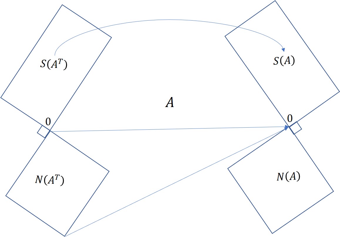
It maps a vector in the row space, i.e., the subspace spanned by row vectors of $A$, to a vector in the column space, the subspace spanned by column vectors of $A$.

Define

1. $S(A^T) = \{ \sum_{i = 1}^n \lambda_i A[i,:] : \lambda_i \in \mathbb{R}, \forall i \in [n] \}$, which we call the row space of $A$.

2. $N(A^T) = \{ x \in \mathbb{R}^m, s.t., Ax = 0\}$, the subspace perpendicular to $S(A^T)$.

3. $S(A) = \{ \sum_{i = 1}^m \lambda_i A[:,i] : \lambda_i \in \mathbb{R}, \forall i \in [m] \}$, the columns space of $A$.

4. $N(A)$ the space perpendicular to $S(A)$.

Note that $S(A^T)$ and $S(A)$ has the same dimension $r$. For any $x \in \mathbb{R}^n$, we can write $x = y + z$, such that $y \in S(A^T)$ and $z \in N(A^T)$. The operation $Ax = Ay + Az$, takes the $y$ component to a vector in $S(A)$ and the $z$ component to point $0$, as illustrated by the figure.

Singular Vector Decomposition

Singular vector decomposition aims to find

1. an orthonormal basis $\{ v_1, v_2, ..., v_r \}$ for $S(A^T)$,
2. and an orthogonal base $\{ u_1, u_2, ..., u_r \}$ for $S(A)$,
3. such that $f(v_i) = A v_i = \sigma_i u_i$ for all $i \in [r]$ and $\sigma_1 \ge \sigma_2 \ge ... \ge \sigma_r > 0$.

When restricted to the sets $\{ v_1, v_2, ..., v_r \}$ and $\{ u_1, u_2, ..., u_r \}$, $f$ is a bijection.

If we write $V = [v_1, v_2, ..., v_r]$,

and $U = [u_1, u_2, ..., u_r]$, then

As the columns of $V$ are orthonormal vectors, it is invertible and $V^{-1} = V^T$. Hence

Equivalently, it holds that

Further,

which implies that

The $v_i$'s and $u_i$'s are eigenvectors of $A^T A$ and $A A^T$ respectively.

EXISTENCE

The key is $A^T A$, which is semi-positive. Since

$A^T A$ and $A$ has the rank $r$, the same null space and hence the same row space. Further, as $A^T A$ is semi-positive, it has $r$ positive eigenvalue. Denote the eigenvalues of $A^TA$ in decreasing order as $\lambda_1 \ge \lambda_2 \ge ... \ge \lambda_r > 0$ and the corresponding (unit length) eigenvectors as $v_1, v_2, ..., v_r$. The $v_i$'s are orthogonal, as

• For $i \neq j$, $v_i^T A^T A v_j = \lambda_i v_i^T v_j = \lambda_j v_i^T v_j$. As $\lambda_i \neq \lambda_j$, $v_i^T v_j = 0$.

They constitute an orthogonal base of the row space of $A^T A$ and the row space $A$.

Now we use the $v_i$'s to search for $u_i$'s as follows: let $\sigma = \sqrt{\lambda_i}$, we claim that

are orthonormal.

1. The $u_i$'s are orthogonal: $u_i^T u_j = \frac{1}{\sigma_i \sigma_j} v_i^T A^T A v_j = \frac{\sigma_j^2 }{\sigma_i \sigma_j} v_i^T v_j = 0$
2. The $u_i$'s are unite vectors: $u_i^T u_i = \frac{1}{\sigma_i^2} v_i^T A^T A v_i = 1$

Hence $u_i$'s constitutes an orthonormal basis. As the columns of $A$ has dimension $r$, the $u_i$'s covers the entire columns space. This completes the proof.
$\blacksquare$

GEOMETRIC INTERPRETATION

To understand the geometry of SVD, we first extend the matrix $V$ to an orthogonal base in $\mathbb{R}^n$ and $U$ to an orthogonal base in $\mathbb{R}^m$. By adding proper zero rows and columns to $\Sigma$, we still have $A = U \Sigma V^T$.

Now, the transformation $f(x)$ is decomposed into three steps:

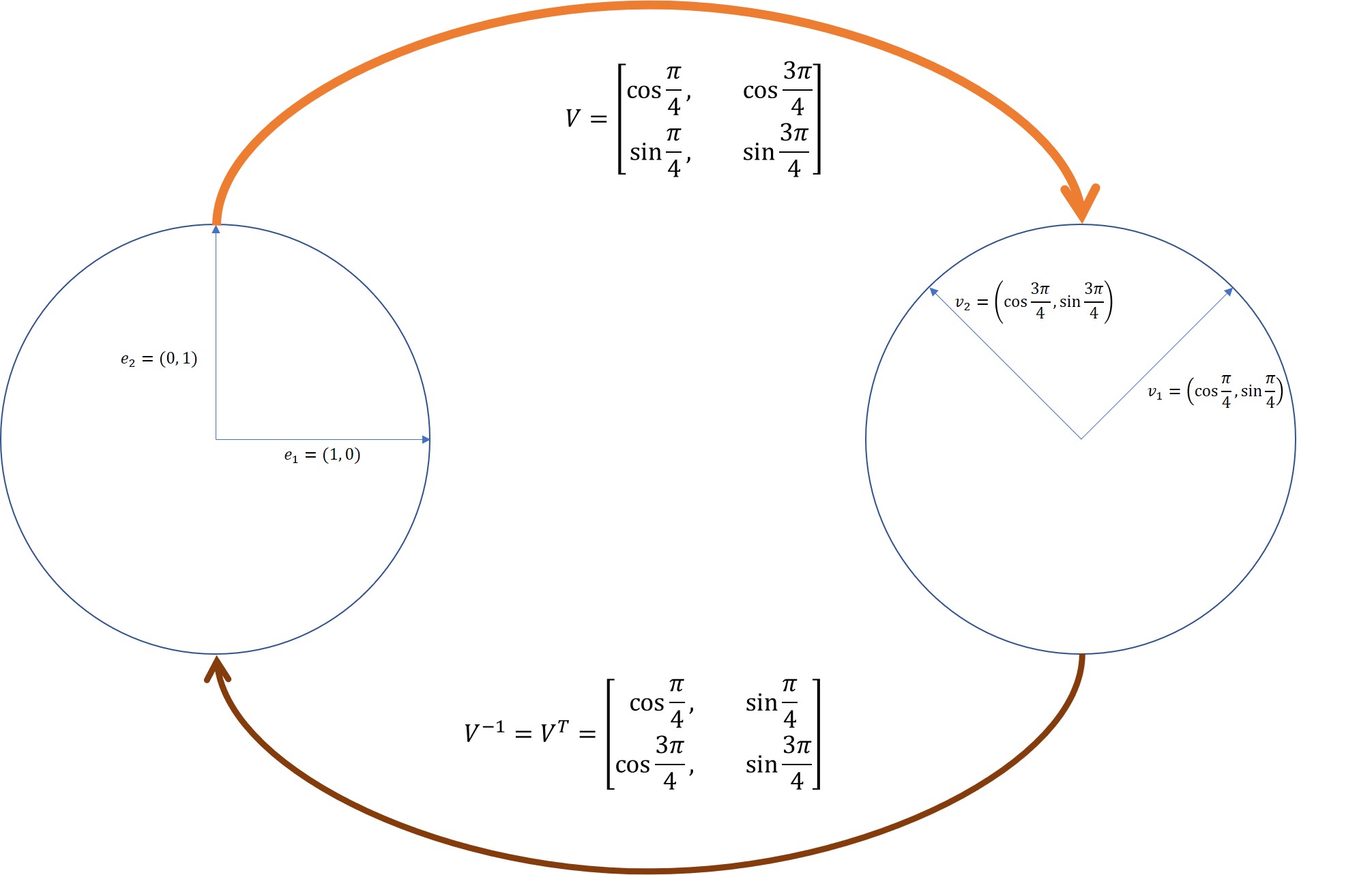
It suffices to under the effect of multiplying an orthogonal matrix $V$. It is indeed a rotation. To see this, multiply $V$ by $e_i$ gives $v_i$, i.e., $V e_i = v_i$, for all for $i \in [n]$. Therefore, $V$ takes the orthogonal base $I = [e_1, e_2, ..., e_n]$ to the orthogonal base $V = [v_1, v_2, ..., v_n]$.

Note that the inverse $V^{-1}$ of $V$ is also an orthogonal matrix and hence a rotation. Indeed it rotates the orthogonal base $V = [v_1, v_2, ..., v_n]$ back to $I = [e_1, e_2, ..., e_n]$. To understand this, observe that $V^{-1} = V^T$. For arbitrary $v_i$, we have $V^T v_i = e_i$.

Therefore, $V^T x$ corresponds to a rotation, in the reverse direction to the one defined by $V$.

Next, the matrix $\Sigma$ scales the $i$-th dimension of $V^T x$ by $\sigma_i$, for all $i \in [n]$. Combined with the first step, if $x = v_i$, then it is first rotation to the direction $e_i$, then scaled by a factor $\sigma_i$.

Finally, $U$ is an orthogonal matrix and corresponds to another rotation, which take $e_i \in \mathbb{R}^m$ to a vector $u_i$.

Corollary: Define the Frobenius norm of a matrix $A$ as

Then $\Vert A\Vert _F^2 = \Vert \Sigma\Vert ^2 = \sum_{i = 1}^r \sigma_i^2$.

Proof: Note that rotating the vectors do not change their distance from the origin. Recall that $U^T$ and $V$ are both rotations. Hence $\Vert A\Vert _F^2 = \Vert AV\Vert _F^2 = \Vert U^T A V\Vert _F^2 = \Vert U^T U \Sigma V^T V\Vert _F^2= \Vert \Sigma\Vert _F^2$.

$\square$.

APPLICATIONS

An important property of the $v_i$ is that

1. $v_1 = \arg\max_{v \in \mathbb{R}^n, \Vert v\Vert = 1} \Vert Av\Vert$.
2. $v_2 = \arg\max_{v \in \mathbb{R}^n, \Vert v\Vert = 1, v \perp v_1} \Vert Av \Vert$.
3. ...
4. $v_r = \arg\max_{v \in \mathbb{R}^n, \Vert v\Vert = 1, v \perp v_1, v \perp v_2, ..., v \perp v_{r - 1}} \Vert Av \Vert$

Proof: For any $v \in \mathbb{R}^n, \Vert v\Vert = 1$, we can write $v = \sum_{i = 1}^n a_i v_i$, where $\sum_{i = 1}^n a_i^2 = 1$, since $v_i$'s are an orthogonal base. Then

which is maximized to $\sigma_1^2$ when $a_1 = 1$ and $a_i = 0, i \ge 2$. Hence (1) is proved.

Similarly, when $\Vert v\Vert = 1, v \perp v_1, v_2, ..., v_k$ for some $k < r$, then $a_1 = a_2 = ... a_k = 0$, and $v = \sum_{i = k + 1}^r a_i v_i$.

which achieves maximum when $a_{k + 1} = 1$ and $a_i = 0, i > k + 1$. In this case $v = v_{k + 1}$.

Best Fit $k$ subspace

An implication is that, the subspace space $V_k$ spanned by $(v_1, v_2, ..., v_k)$, is the best $k$-dimension subspace of $\mathbb{R}^n$ that fits the row vectors of $A$, namely, $A[1, :], A[2, :], ..., A[m, :]$. Here fits mean the sum of the square of the perpendicular distance from the row vector to their projections on the subspace is minimized. Denote $S$ any subspace of $\mathbb{R}^n$, then for $v \in \mathbb{R}^n$, we can decompose $v$ into two part: the part $v_S$ that is within $S$ and the part $v_{S_\perp}$ perpendicular to $S$. Then

Minimizing $\Vert v_{S_\perp}\Vert ^2$ is equivalent to maximizing $\Vert v_{S}\Vert ^2$. The subspace space by $(v_1, v_2, ..., v_k)$ is the subspace that maximize the sum of the squares of the projections of row vectors to the subspace.

We prove this by induction. When $k = 1$, the proof holds trivially by the definition of $v_1$. In particular, $A v_1$ is the lengths of the projections of the row to the line that go through $v_1$, since $v_1$ is a unit vector. Further, the corresponding projected vectors in $\mathbb{R}^n$ are

For general $k$, by induction hypothesis $V_{k - 1}$ is the best $k-1$ dimension space that fit rows of $A$. Denote $N(V_{k -1})$ the subspace that is perpendicular to $V_{k - 1}$, which has dimension $n - k + 1$. For any $k$ dimensional subspace $S \cap N(V_{k - 1}) \neq \emptyset$, since $dim(S) + dim(N(V_{k - 1})) = k + n - k + 1 \ge n$. Let $s_k \in S \cap N(V_{k - 1})$ be a unit vector. By the definition of $v_k$, we have

Now we can extend $s_k$ to a base of $S$, denoted as $s_1, s_2, ..., s_k$. By induction hypothesis, it holds

Hence

But the former is exactly sum of the squares of the lengths of the projections to $V_k$ and the later is the one to $S$. Finally, we mention that the projection of $A$ to $V_k$ is given by

Corollary 1. For any rank $k$ matrix $B$, we have

Intuitively, if we view square root of the sum of square distance of row vectors to the origin (note that the origin can be viewed as a zero dimension subspace.)

Corollary 2. Define the 2-norm of a matrix $A$ as

The $2$-norm is the square root of the maximum sum of squares of the projections of the row vectors to a one dimension subspace. Then an implication of the SVD is that, for any rank $k$ matrix $B$, we have

Proof: First note that for $v = \sum_{i = 1}^r a_i v_i$, such that $\sum_{i = 1}^k a_i^2 = 1$,

it is maximized when $a_{k + 1} = 1$ and $\Vert A - A_k\Vert _2 = \sigma_{k + 1}$. Now, as $dim(A_{k + 1}) + dim(N(B^T)) = k + 1 + n - k \ge n$, $\exists v \in \mathbb{R}^n$, such that $Bv = 0$ and $v = \sum_{i = 1}^{k + 1} a_i v_i$ and $\Vert v\Vert = 1$. Now

which finishes our proof.

Computing SVD

If suffices to compute the eigenvectors and eigenvalues of $A^T A$, i.e., $\sigma_i^2$'s and $v_i$'s. In the simplest case, $\sigma_1 > \sigma_2 \ge \sigma_3 \ge ... \ge \sigma_r$, then we can take powers of $A^T A$,

Dividing the matrix by $\sigma_1^{2k}$,

The second part converges to 0 as $k \rightarrow \infty$. Then for any vector $v$ that is not perpendicular to $v_1$, we have

which is a multiple of $v_1$. Normalizing the vector recovers $v_1$.

When there is a tie of the largest eigenvalues, that is $\sigma_1 = \sigma_2 = ... = \sigma_t$ for some $t < r$, and suppose that $v$ is not perpendicular to $v_1, v_2, ..., v_t$ simultaneously, then

Suppose we are satisfied with this result, we still need to address two problems.

1. We use $\sigma_1^{2k}$ to normalize the resulting vector, which is unknown.
2. How can we find a vector $v$ that is not perpendicular to all $v_1, .., v_t$ simultaneously, i.e., its projection to $V_t$ is not zero.

We defer the discussion of the first issue. As for the second issue, we tackle the problem for picking a vector $v$ uniformly at random from the $n$-dimension unit ball, and then normalize it by $v / \Vert v\Vert $, in the hope that it is a "good" vector.

Lemma: With probability at least $1 / 2$, that $v^T v_1 \ge 1 /\sqrt{n}$.

Proof: By symmetry of the $n$-dimension unit ball, it suffices to show that for an arbitrary given fixed direction, the projection of $v$ to that direction is at least $1 / 4 \sqrt n$ with probability $1 / 2$. For convenience, we choose this direction to be $e_1$.

Denote the volume of an $n$-dimensional unit ball as $V(n)$.

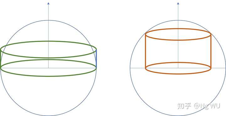
Now, we would like to use two cylinders to estimate the probability of $|e_1 ^T v| / \Vert v\Vert \le \frac{1}{4 \sqrt n}$.

Note that the points $\{v \}$ inside the ball with $e_1^T v / \Vert v\Vert \le \frac{1}{4 \sqrt n}$ is completely contained in a cylinder centered in the equator, with radius one and height $\frac{1}{4 \sqrt n}$ that is parallel to $e_1$. Its volume is given by $\frac{1}{4 \sqrt n} V(n - 1)$. Hence:

On the other hand, we can use a cylinder centered at the equator to lower bound the volume of $n$-dimension unit ball. The cylinder is inside the ball, with height $2\frac{1}{\sqrt n}$ and radius $(1 - (\frac{1}{ \sqrt n})^2)^{1/ 2}$ . Therefore,

Note that $(1 - \frac{1}{n})^n$ increases with $n$, and for $n \ge 2$, $(1 - \frac{1}{n})^n \ge \frac{1}{4}$ and $\left( 1 - \frac{1}{n} \right)^{n / 2} \ge \frac{1}{2}$

$\square$

Theorem After $\frac{1}{\epsilon} \ln \frac{n}{\epsilon}$ iterations, we can obtain a vector whose component that is perpendicular to $V_t$ is at most $\epsilon$ fraction of its square length, with probability at least $\frac{1}{2}$.

Proof: If $\sigma_i < (1 - \epsilon) \sigma_1$, then

Denote $\sigma_1 = \sigma_2 = ... = \sigma_t$ for some $t < r$ the largest singular values. By the previous lemma, we pick a $v$ from the unit ball at random, and take $v \leftarrow v / \Vert v\Vert $. Denote $v = \sum_{i = 1}^n {a_i} v_i$, then with probability at least $1/ 2$ we have $\sqrt{ \sum_{i = 1}^t a_i^2} \ge \frac{1}{4 \sqrt n}$. On the other hand, $v$ is a unit vector, hence $\sum_{i = 1}^n a_i^2 = 1$. Therefore, $\sum_{i = t + 1}^n a_i^2 \le 1 - \frac{1}{16 n}$

Now

For the second term

For the first term

If we take $k = O( \frac{1}{\epsilon} \ln \frac{n}{\epsilon})$, then the second term is at most $\epsilon$ fraction of the first term.

Remark: picking a point uniformly at random can be done as follows: first pick a point $v$ uniformly at random from the high dimension cube: $[-1, 1]^n$, then checks whether the point is inside the ball ($\Vert v\Vert < 1$). This however, could suffers from efficiency problem as the volume of the ball approaches to $0$ as the number of dimension increases. More efficient sampling method is needed. But it is not the current focus of this article.

Reference

[1]. GILBERT STRANG, Introduction to Linear Algebra.

[2]. Venkatesan Guruswami and Ravi Kannan, Note 2, Singular Value Decomposition, 15-496/15-859X: Computer Science Theory for the Information Age, Spring 2012, CMU