Suppose we have a set of facilities F and a set of clients C,
and would like to open a subset of facilities to serve the clients.
The cost consists of two parts:
one for opening the selected facilities;
one for connecting each client to its nearest facility.
Formally, denote fi the cost of facility i∈F and du,i the distance from a client u∈C to a facility i∈F.
Further, we assume that the distances satisfy the following constraint:
dv,i≤dv,j+du,j+du,i,∀u,v∈C,i,j∈F.
Let S⊆F be a subset of facilities.
The cost of S is given by
i∈S∑fi+u∈C∑i∈Smindu,i
The problem is to find a set S that minimizes this cost.
Linear Programming
The linear program for the problem is given as follows:
The first constraint says that each client is assigned to at least one facility.
The second one says that a facility must be (fractionally) open if there is a client assigned to it.
Weak Duality ⟹ Dual Program
Let αu be the dual variable associated with constraint (1) and βu,i be the one with constraint (2).
We want the following inequalities, called weak duality, to hold:
When such inequalities hold, ∑u∈Cαu constitutes a lower bound for cost of the primal program.
The problem of obtaining a tightest such lower bound, under the constraints under which the above inequalities hold, gives the dual program:
Here we give a more intuitive way of deriving the dual.
First, observe that ∑u∈Cmini∈Fdu,i is a trivial lower bound of the primal programming.
In this case, each client is assigned to its nearest facility.
However we ignore facility cost entirely.
To incorporate the facility cost, for each facility i we divide its cost fi among the clients, such that client u needs to pay βu,i if it is assigned facility i.
Note that βu,i can be arbitrary non-negative number as long as it satisfies that ∑u∈Cβu,i=fi for all i∈F.
Theorem. For each subset S⊆F, let μ:C→S be the function defined by
Then ∑u∈Cαu constitutes a lower bound for the cost of each solution for the primal LP.
In particular, it is a lower bound of the cost of the optimal integral solution S∗ (its corresponding assignment function is denoted as μ∗):
u∈C∑αu≤i∈S∗∑fi+u∈S∗∑i∈Smindu,i.
The problem of determining a set of βu,i's that maximizes the lower bound ∑u∈Cαu gives the dual program.
Let x∗,y∗ and α∗,β∗ be the optimal primal and dual solutions, respectively.
For these set of variables, weak duality holds with equalities. By complementary slackness, it holds that
αu∗=0 or ∑i∈Fxu,i∗=1
βu,i∗=0 or yi∗−xu,i∗=0
and
αu∗−βu,i∗=du,i or xu,i∗=0
∑u∈Cβu,i∗=fi or yi∗=0
Deterministic Rounding [1]
4-Approximation Algorithm
We show how to pick a good subset S⊂F based on the optimal solutions x∗,y∗, α∗ and β∗.
First we construct a graph G=(V,E) based on the x∗.
Definition. A derived graph from the optimal LP consists of the follows:
The vertex set V=F∪C;
The undirected edge set E={(u,i):xu,i∗>0,∀i∈F,u∈C}, i.e., the edge set E consists of client-facility pairs (u,i) for which xu,i∗>0.
In the graph G, the neighbors a client u∈C can only be facilities.
Definition. For each u∈C, let N(u) be the set of facilities adjacent to u in G.
Similarly, we define two-hop neighbors of a client C, as the client who connects to u via a intermediate facility.
Definition. For a client u∈C, its two hop neighbors are the set of clients v whose distance to u is at most 2:
N2(u)={v∈C:N(u)∩N(v)=∅}.
Note that u∈N2(u).
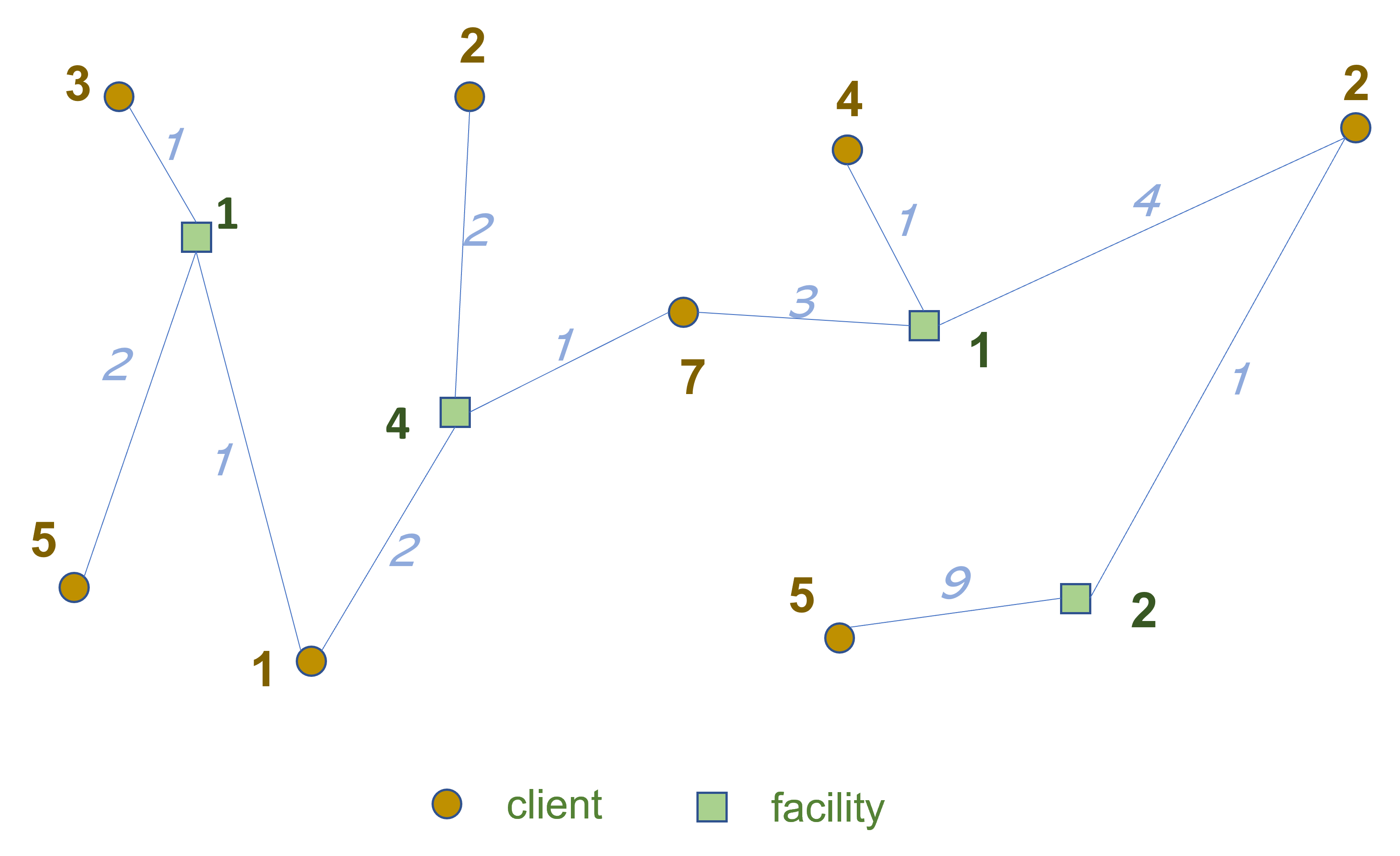
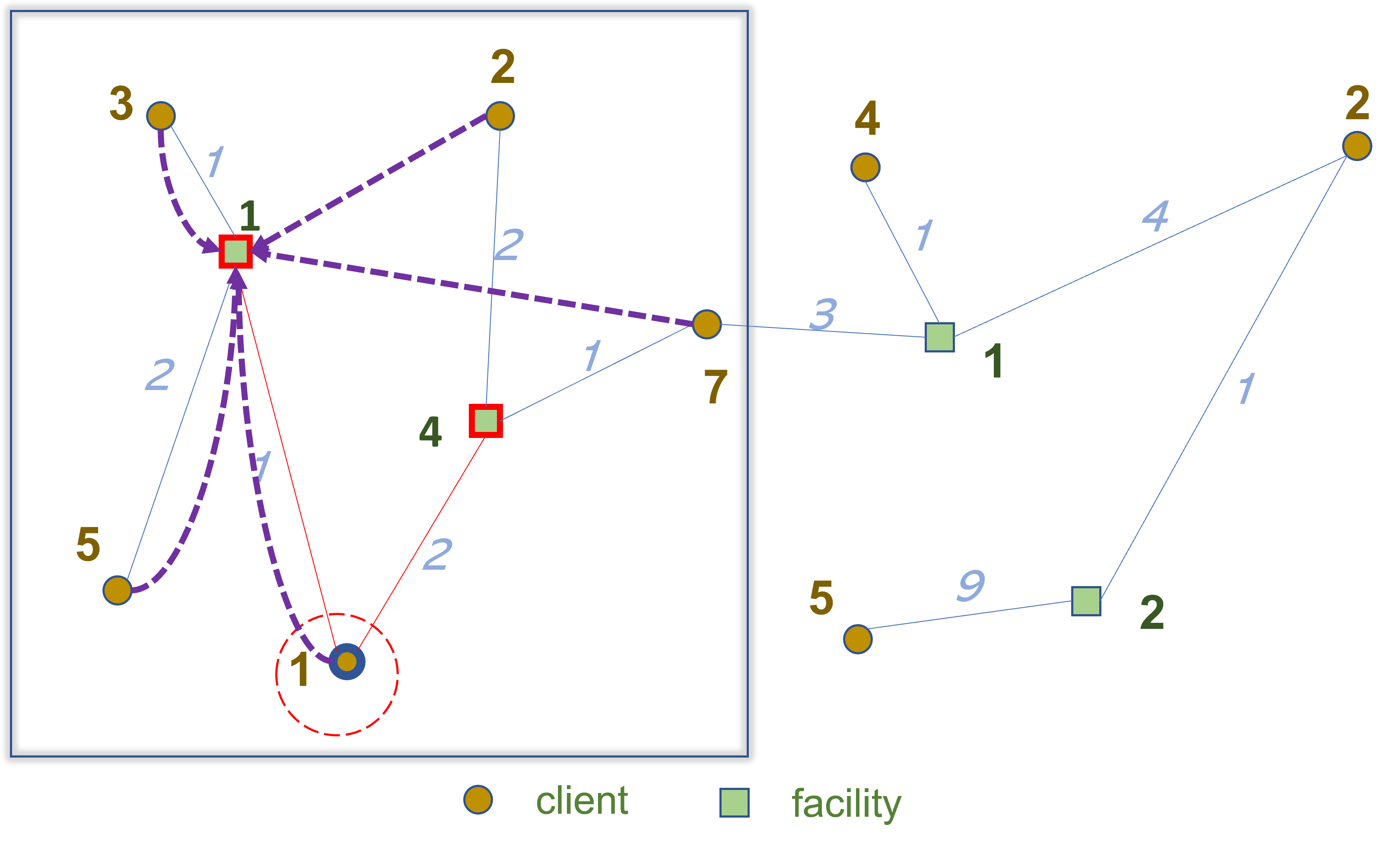
Below is an example. The cycles represent clients and the squares are for facilities. Associated each client and each facility are the αu∗ value and opening cost respectively.
An important property of this graph is that
Property. If (u,i)∈E, then xu,i∗>0, which implies that αu∗=du,i+βu,i∗ by complementary slackness.
It concludes that αu∗≥du,i if there is an edge (u,i) in G.
The following is the first constant factor approximation algorithm for the un-capacitated facility location problem, proposed in 1997 [1].
Algorithm 1
S←∅
U←C;B←∅
whileU=∅do
u←v∈Uargminαv∗
iu←i∈N(u)argminfi
U←U∖N2(u)
B←B∪{u}
S←S∪{iu}
It is important that at each iteration, when a client u is chosen, all vertices clients in N2(u) are removed from U.
This guarantees that clients in B has non-overlapping neighbors, i.e.,
N(u)∩N(v)=∅,∀u,v∈B.
Consider the assignment scheme in which, instead of assigning each client to its nearest facility in S, at each iteration, we assign clients in N2(u) to the chosen facility iu.
Then each iteration of the algorithm creates a clusters, which contains three kinds of vertices:
The selected client u with minimum αu∗.
All u's neighboring facilities.
All un-assigned clients neighboring to these facilities.
Such clusters are non-overlapping.
The example above shows one iteration of the algorithm.
The vertex with minimum value of αu∗ (i.e. 1) is opened, highlighted by the red cycle.
There are two facilities connected to it, the cheap opening cost of which is 1.
Then all un-assigned clients neighboring these two facilities are assigned to the cost 1 facility, as shown by the purple dashed arrows.
It is left to analyze the cost of the solution returned.
Theorem. The facility cost of Algorithm 1 is at most OPT.
Proof.
At each iteration, a client u is selected. In the primal LP, constraint (1) requires that
i∈F∑xu,i∗≥1
Note that although u can assigned to a facility fractionally, the total amount of assignment must be at least 1.
Further, although a facility can be fractionally open in primal LP, the constraint (2)
yi∗≥xu,i∗
implies that the open amount must be at least the amount a client assign to it.
We conclude that
The neighbor sets N(u)'s of the selected clients u∈B are disjoint.
Therefore, summing over u∈B, the total facility cost is bounded by
u∈B∑i∈N(u)∑yi∗fi≤i∈F∑yi∗fi≤OPT.
Theorem. The connection cost of Algorithm 1 is at most 3⋅OPT.
Proof.
Now we analyze the assignment cost.
Case One. If u∈B, then it is selected by the algorithm, and iu≐argmini∈N(u)fi belongs to S.
Therefore,
du,S≐argi∈Smindu,i≤di,iu≤αu∗.
Case Two. If v∈/B, then v∈N2(u) for some u∈B.
Since v∈N2(u), there exists some facility j∈N(v)∩N(u).
By triangle inequality, we have
dv,iu≤dv,j+du,j+dv,iu≤αv∗+αu∗+αu∗≤3αv∗
The last inequality holds since αu∗≤αv∗.
□
Combing assignment cost and facility cost, Algorithm 1 is 4-approximation.
How happy are we with the 4-approximation algorithm? Probably not. In the previous example, when a facility is opened, only one client contributes to its opening cost.
However, in the primal solution, many other clients assigned to it do not contribute to the opening cost, which implies that the current analysis may not be tight.
Randomized Rounding [3]
3-Approximation Rounding
In the section, we improve the approximation ratio of 4 to an expected value of 3.
In the previous rounding, we bound the opening cost as
u∈B∑i∈N(u)minfi≤OPT
which is not tight.
Define the assignment cost for client u in the optimal primal LP solution as Au=∑i∈Fxu,i∗du,i.
Indeed, it is affordable to bound
u∈B∑i∈N(u)∑xu,i∗fi+u∈B∑Au≤OPT
It is possible to devise a randomized rounding algorithm that incorporates this cost and improve the approximation ratio to 3.
The only differences compared to the first rounding algorithm are
We pick a client that minimize αu∗+Au;
We pick a facility with probability xu,i∗.
Below is the algorithm.
Algorithm 2
S←∅
U←C;B←∅
whileU=∅do
u←v∈Uargmin(αv∗+Av)
Pr[iu←i]=xu,i∗,∀i∈N(u)
U←U∖N2(u)
B←B∪{u}
S←S∪{iu}
Facility Cost
The analysis of expected facility cost is almost the same as before. It is guaranteed that
N(u)∩N(v)=∅,∀u,v∈N(u).
Therefore, the expected opening cost is bounded by
Case One. If v∈/B, then there exists u∈B, s.t., v∈N2(u).
Then there exists some facility j∈N(u)∩N(v).
By triangle inequality, the expected connection cost is at most
Remark: there is still room for improvement.
When a client u is selected and a facility i is sampled, v∈N2(u) is assigned to i.
On the other hand, v itself may contributes to the opening cost of some other facility not open.
To make the expected opening cost tight, we may consider opening facilities directly with respect to probability yi∗.
(1+3/e)-Approximation Rounding [3]
In the previous analysis, we see that a facility may be under-sampled.
There are two reasons for this:
For a facility i, ∃u∈N(i) such that u∈B. When u is selected, facility i is sampled with probability xu,i∗, which might be smaller than yi∗.
For a facility i, none of its clients u∈N(i) is selected, therefore i is never sampled.
To fix theses issues and based on Algorithm2, we have the following algorithm.
The algorithm presented here is a modified version of the one proposed in [3], but guided the same philosophy.
Algorithm 3:
T←F
k←0
S1,S2,S3←∅
while there exists un-assigned client do
k←k+1
Let uk be the unassigned one with smallest αu∗
Open exactly one facility ik∈N(uk) with probability xu,i∗
S1←S1∪{ik}
For each i∈N(uk)−{ik}
Open i with probability (yi∗−xu,i∗)/(1−xu,i∗)
S2←S2∪{i}
T←T−N(uk)
Assign v to ik, for each v∈N2(uk)
for each facility i∈T
Open i with probability yi∗
S3←S3∪{i}
Re-assign each u∈C to its nearest open facility.
When the algorithm stops, denote S=S1∪S2∪S3 the set of open facilities and B={u1,u2,...,u∣B∣} the set of selected clients by line 6.
The following lemma shows that Algorithm 3 fully samples each facility and therefore never loses to Algorithm 1.
Facility Cost
Lemma 1. For each i∈F, it is opened with probability yi∗.
Proof. Note the facilities are not open independently. The claim is trivially true if a facility is is sampled in line 10. Otherwise, ∃u∈B, s.t., i∈N(u). The probability of i being open is
xu,i∗+(1−xu,i∗)⋅1−xu,i∗yi∗−xu,i∗=yi∗.
■
Corollary. By linearity of expectation, the expected facility opening cost is ∑i∈Fyi∗fi.
Connection Cost
What is not trivial is the analysis of the assignment cost.
Given S, assigning u∈C to its nearest facility in S minimizes the assignment cost.
To bound this cost, we investigate a sub-optimal assignment based on S.
For each u∈C we select a subset S(u)⊆S and assign it to a closest facility in S(u).
This leads to a possibly increase in the expected assignment cost.
Let Z be the random variable of the assignment cost for client u and Xi (i∈N(u)) be the indicator random variable of i being in S(u).
As when none of the facility in N(u) is selected into S(u), then assignment cost is bounded by 3⋅αu∗, the value of Z is therefore at most
Note that the inequality here may not be tight, as we replace the min operation into ∑.
But it suffices to prove the expected approximation ratio.
When combined with the expected facility opening cost, we know that total expected cost is bounded by
The S(u) is generated as follows.
If u∈B, then we let S(u)=S.
Otherwise, we initialize S(u) with S−N(u), and for facility i∈N(u)∩S, we perform some carefully designed operations to ensure that Pr[i∈S(u)]=xu,i∗.
If i∈S3, we keep it in S(u) with probability yi∗xu,i∗. Therefore,Pr[i∈S(u)]=Pr[i∈S(u)∣i∈S]⋅Pr[i∈S]=xu,i∗
Otherwise, ∃uk∈B, such that i∈N(uk). There are two possible cases
Case 1: xi,uk∗≥xu,i∗, the probability of selecting i is defined as follows:
It is left to show that Pr[I[Xi=0,∀i∈N(u)]=1]≤1/e.
For u∈B, this holds trivially.
If not, we prove the following lemma.
Lemma 2. For any client u∈C∖B, the probability that none of facility in N(u) belongs to S(u) is bounded by 1/e.
Proof.
Observe that
N(j1)∪N(j2)∪...∪N(j∣B∣)∪T=F
constitutes a partition of F.
For any client u, define Rk=N(uk)∩N(u), where 1≤k≤∣B∣.
Further, let R∣B∣+1=T∩N(u).
Then {Rk}k∈[∣B∣+1] is a partition of N(u).
Consider facilities in N(uk) (k∈[∣B∣]).
The probability of none of them being in S(u) is
In this section we show a primal-dual algorithm that is purely combinatorial.
Initially we have a set of dual variables αu,u∈C and βu,i,u∈C,i∈F that are set to 0.
Note that they are feasible.
Then we try to optimize this set of variables by increasing all αu,u∈C in parallel until some αu's are blocked.
Why are they blocked? Because the dual constraint
αu≤du,i+βu,i
becomes tight for some client u∈C.
If we increase αu further, the variables are no longer dual feasible.
However, we can modify our strategy by increasing these βu,i simultaneously with αu until facility i is blocked, i.e.,
u∈C∑βu,i=fi.
Definition. For each facility i∈F, define its neighbors N(i) as to be the clients such that αu≥du,i.
The algorithm for constructing the dual variables are given as follows.
Algorithm. Increasing the Dual
U←C: the set of un-blocked clients.
B←∅: the set of blocked facilities.
whileU=∅do
For∀u∈U
Increase all αu (if necessary, βu,i for some i ) simultaneously
Until either
some facility i∈/B is blocked:
B←B∪{i}
U←U∖N(i)
some client u neighbors a blocked facility i∈B:
U←U∖{u}
Question to Ponder. What is the running time for the Dual Variable Increment algorithm.
After running the algorithm above, we get a set of maximal variables which we can't simultaneously increase any more.
It has the following property
Property. Each client u∈C neighbors at least one block facility.
If not, the algorithm will not stop since U is not empty.
Next, we show how to construct an approximate solution from the maximal dual variables.
First we construct a graph G=(V,E) based on the dual LP.
The vertex set V=B∪C.
The edge set E={(u,i):αu≥du,i,u∈C,∀i∈B}.
Moreover, if βu,i>0 for some i∈F, u∈C, we say that u contributes to i.
Definition. For each facility i∈F, let N+(i) be set of clients contributing to it.
Algorithm. Facility Selection
S←∅.
whileB=∅do
Let i∈B be the earliest blocked facility.
S←S∪{i}
// Remove all facilities i′ if ∃u∈C that contributes to both i and i′.
B←B∖{i′∈B:N+(i)∩N+(i′)=∅}.
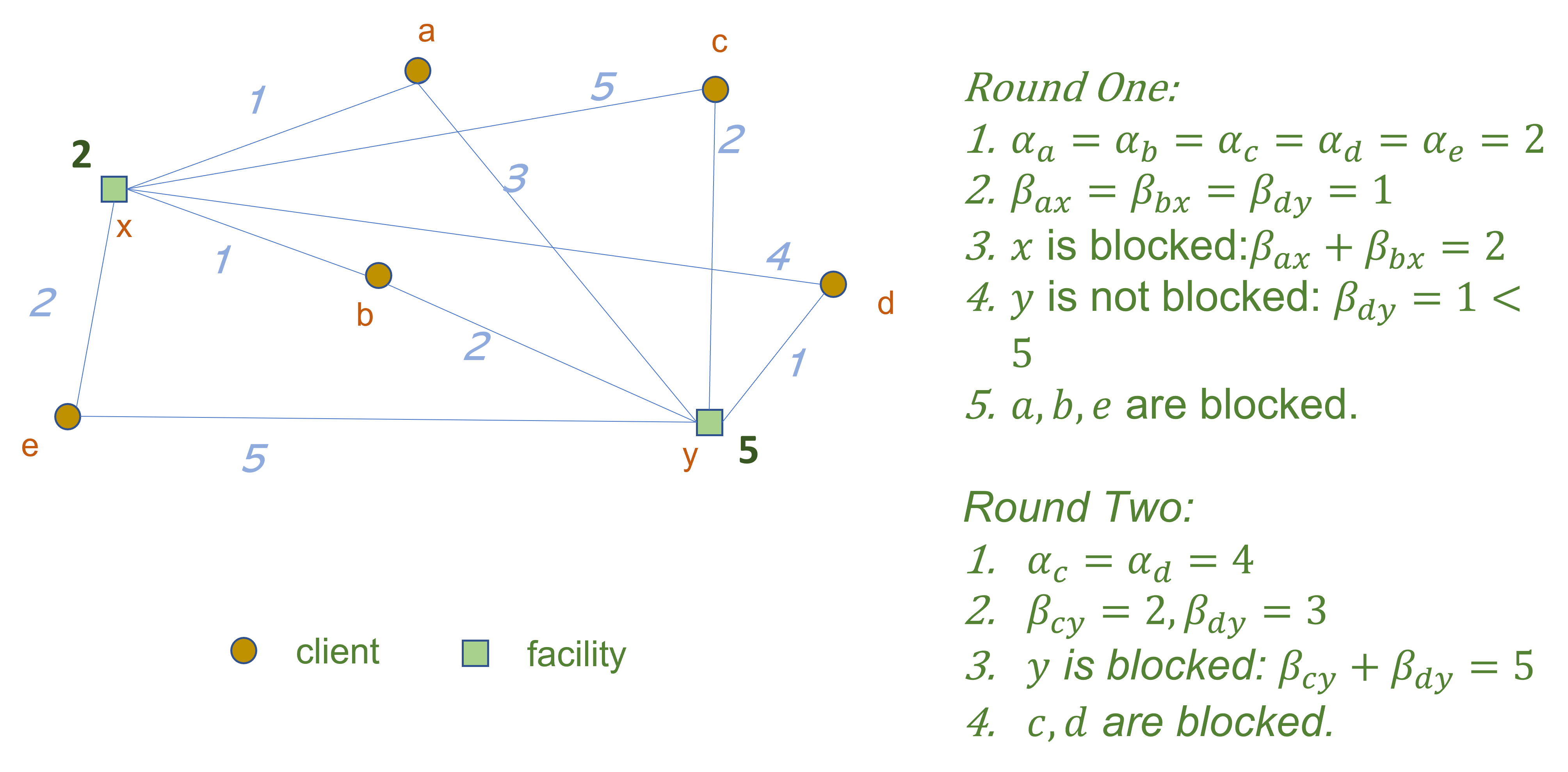
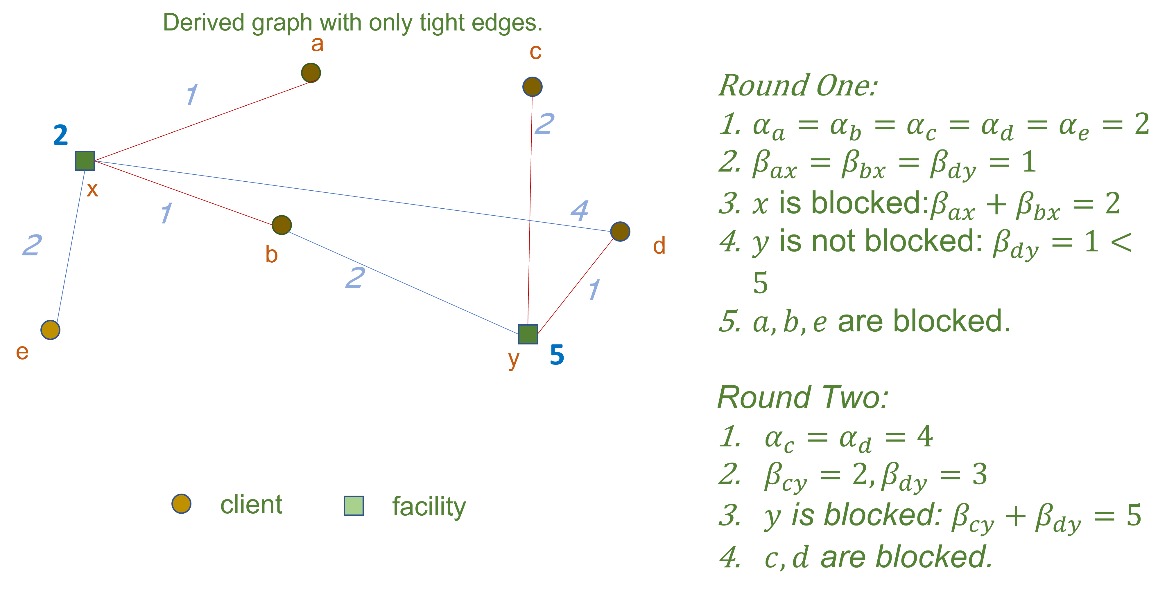
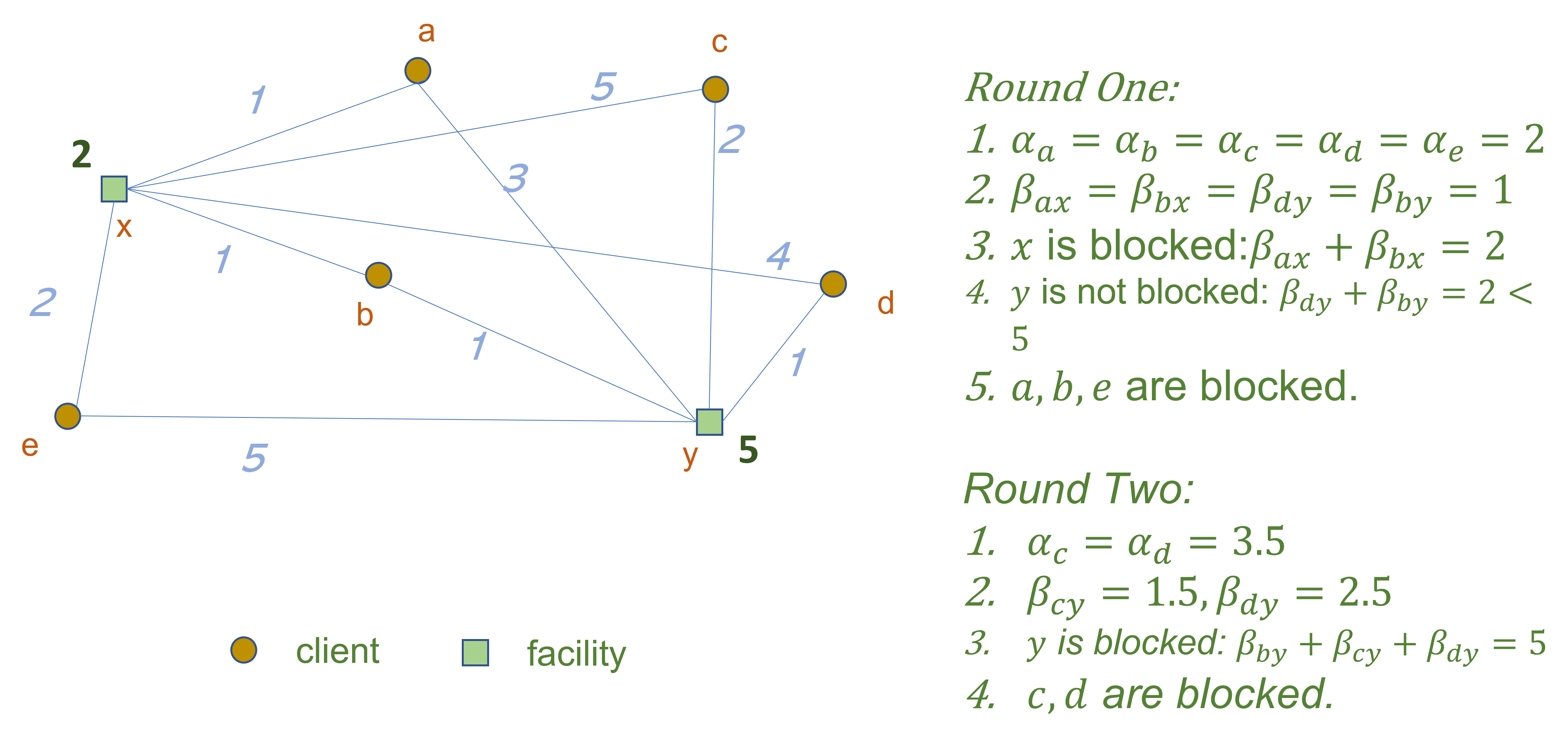
The figure below shows an example of dual variable increment algorithm.
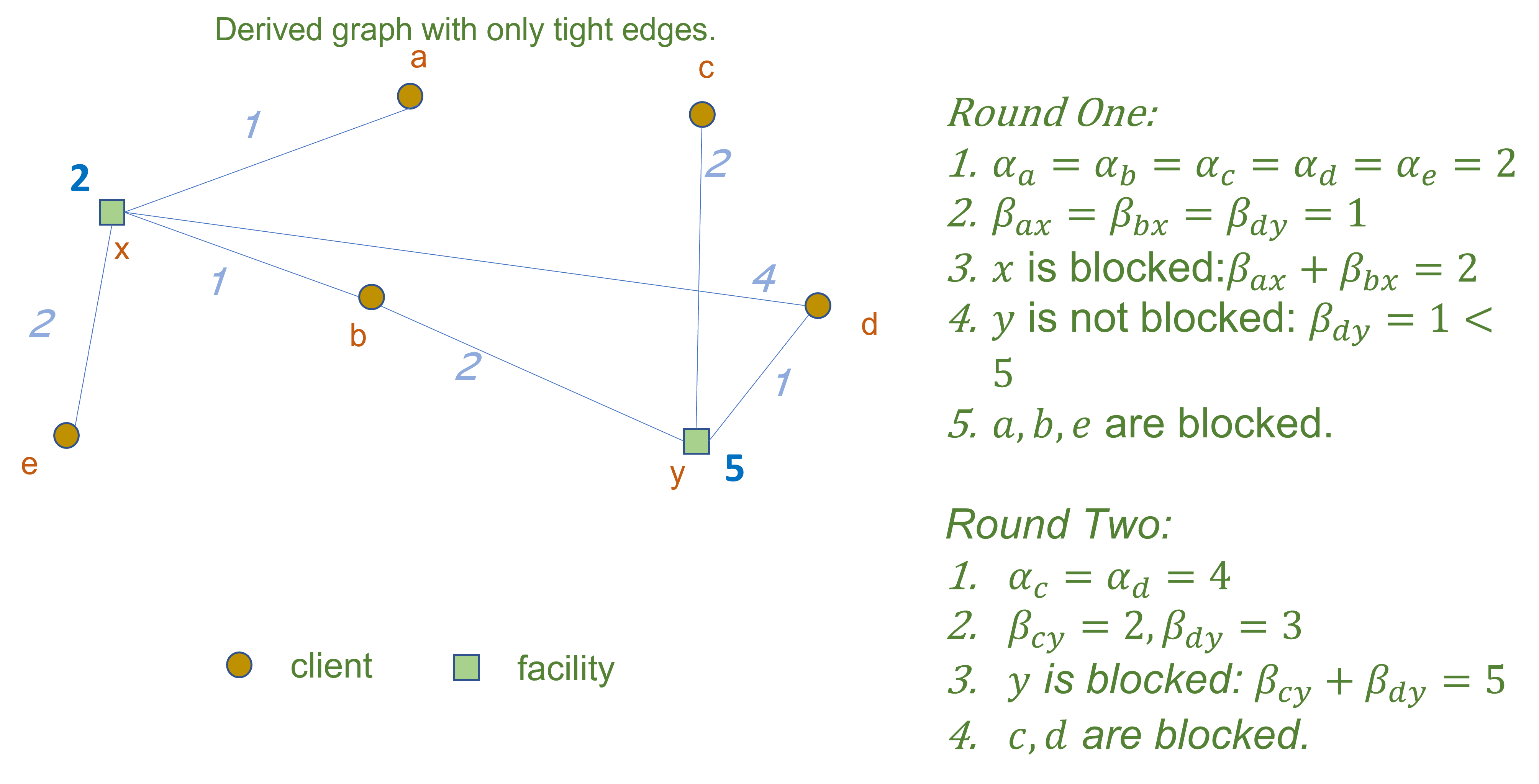
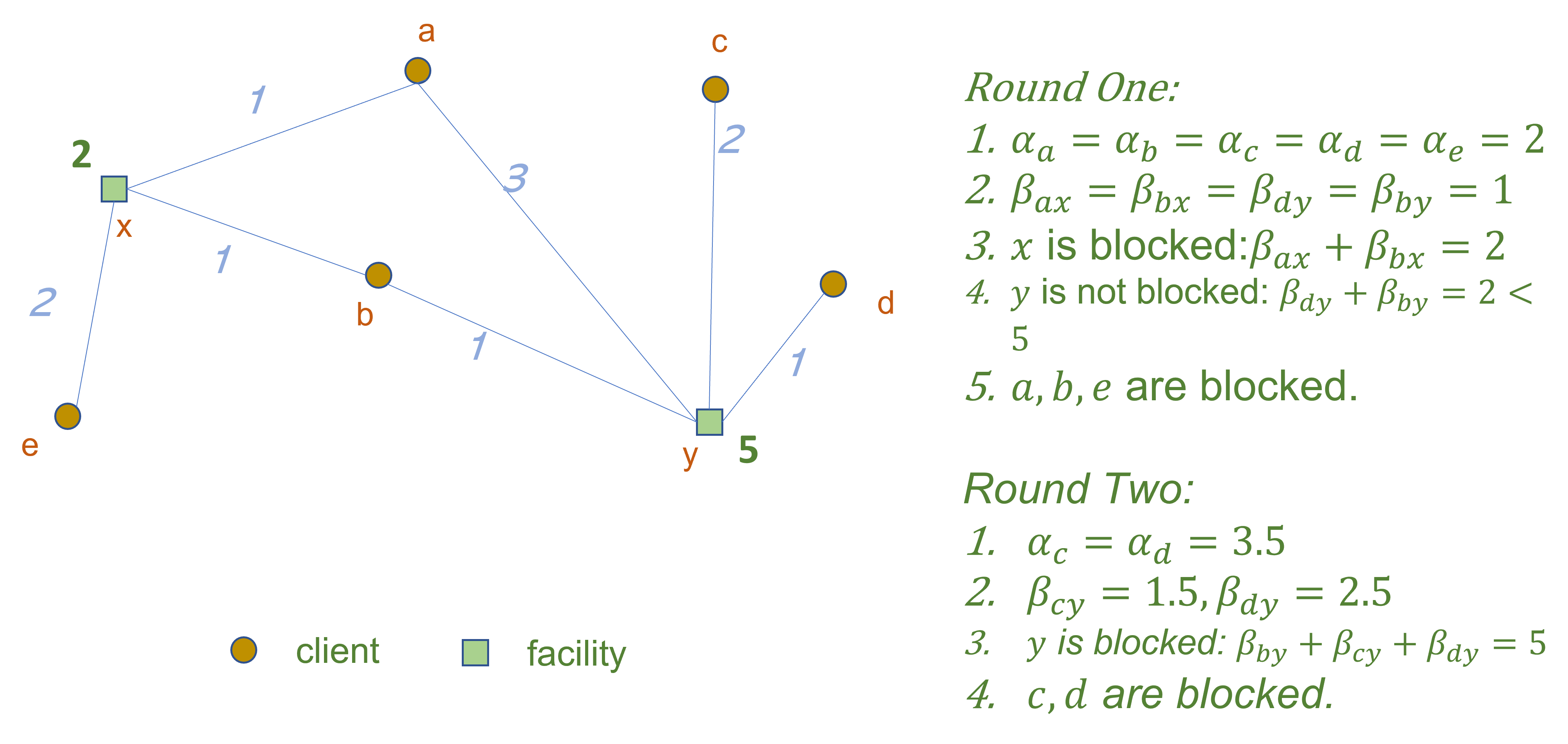
The figure below shows the corresponding derived graph.
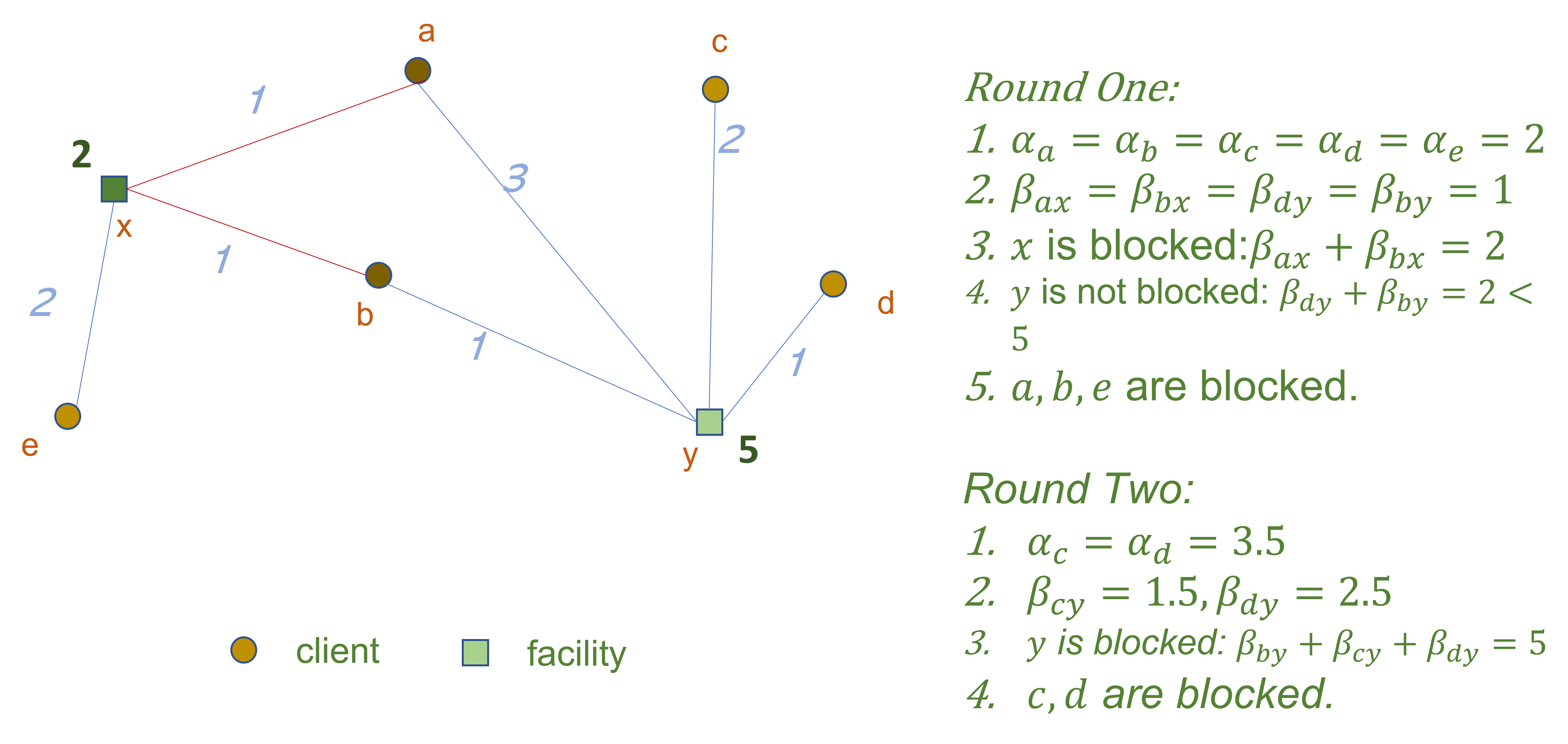
The figure below shows an example of facility selection. The selected facilities are marked with dark green. The clients contributing to theses facilities are connected to them red lines.
Facility Cost
We can show by induction that when a blocked facility is selected, its opening cost is fully covered by all clients contributing to this facility.
Note that if any other blocked facility is connected to any of these clients, it is removed from the candidate set.
Therefore, when a new blocked facility i is selected, the clients in N+(i) can not contribute to any previous selected facility.
The cost of open facilities in S, plus the cost of connecting clients in N+(i) for i∈S, is given by
It is left to consider a client u not in N+(i) for any i∈S.
Case One.u∈N(i) for some i∈S, then the connection cost is
du,i=αu
Case Two.
Otherwise, by the property of the algorithm, we know that there exists a facility i that stops αu from increasing.
The reason that i is not selected is that when some other facility i′ is selected into S, i is removed from the candidate set B because N+(i)∩N+(i′)=∅.
Lemma. Let v∈N+(i)∩N+(i′). Then αv≤αu
Proof.
When i stops αu, since v also contributes to i,
either αv has stopped from increasing or
αv stops simultaneously with u.
□
Therefore, the cost of assigning u to i′ is at most
du,i′≤du,i+dv,i+dv,i′≤αu+2αv≤3αu.
Question to Ponder. What is the running time of the algorithm?
Finally we show another example where the edge weight between (b,y) is changed to 1.
Note that compared to the previous example, only facility x is selected (marked by dark green), because we can use b to contribute only one facility. Now facility y is the one that stops αc and αd from increasing.
Reference
[1] Shmoys DB, Tardos É, Aardal K. Approximation algorithms for facility location problems. InProceedings of the twenty-ninth annual ACM symposium on Theory of computing 1997 May 4 (pp. 265-274).
[2] Jain K, Vazirani VV. Primal-dual approximation algorithms for metric facility location and k-median problems. In 40th annual symposium on foundations of computer science (Cat. No. 99CB37039) 1999 Oct 17 (pp. 2-13). IEEE.
[3] Chudak FA, Shmoys DB. Improved approximation algorithms for the uncapacitated facility location problem. SIAM Journal on Computing. 2003;33(1):1-25.