Every linear program can be converted into Canonical form
maxs.t. cTxAx≤bx≥0
for some c,x∈Rn, A∈Rm×n and b∈Rm.
Dual Program and Weak Duality
Next, we try to construct an upper bound for the optimal solution of this optimization problem, based on its linear constraints.
If y∈Rm and y≥0, then yT(Ax) is called a conic combination of the constraints.
It holds that
yT(Ax)≤yTb.
If y further satisfies the constraint
cT≤yTA,
combining with the fact that x≥0, we get
cTx≤(yTA)x=yT(Ax)≤yTb.
Hence yTb is an upper bound of the optimal value of the original program.
We want the bound to be as tight as possible.
This motivates another linear program:
mins.t. yTbyTA≥cTy≥0
We call the original program the primal and the derived program its dual.
The philosophy behind the dual construction is to combine the primal constraints to obtain a bound of its optimal value.
Corollary. If the primal is unbounded, then the dual is infeasible. If the dual is unbounded, then the primal is infeasible.
In general, the primal may not be given in Canonical form and can be formulated as
To guarantee the second inequality, we require that
yT≥0 (since the constraint Ax+Aˉxˉ+A^x^≤b holds),
yˉT be unconstrained (since the constraint Bx+Bˉxˉ+B^x^=bˉ holds), and
y^T≤0 (since the constraint Cx+Cˉxˉ+C^x^≥b^ holds).
We see that the types of constraints in the primal determine the signs of variables in the dual.
The reverse is also true: the constraints in the dual are determined the signs of variables in the primal.
The first inequality implies that (by proper rearranging):
That gives the first set of constraints the dual variables y, yˉ and y^ need to satisfies, respectively.
We have just seen that the sign of the primal variable determines the type of constraint in the dual.
Of particular interest is the inequality constraint, which we will discuss in details in the next section.
The rules of obtaining dual are summarized as follows:
The strong duality states that, if both primal and dual are feasible, then the objective function values of their optimal solutions are equal.
It follows that the inequalities in weak duality are saturated
cTx=(yTA)x=yT(Ax)=yTb.
Therefore,
(yTA−cT)x=0,yT(b−Ax)=0.
If the primal is in canonical form, then the fact that yTA≥c, x≥0, y≥0, and b−Ax≥0 implies that
where (yTA−cT)i is its i-th coordinate of the vector yTA−cT∈R1×n, and
(b−Ax)j is the j-th coordinate of the vector b−Ax∈Rm×1.
This is known as complementary slackness.
Question to ponder: what is the geometric interpretation of complementary slackness?
Strong Duality
Theorem. Exactly one of the following four cases holds:
Neither the primal nor the dual is feasible.
If both the primal and dual are feasible, then their optimal values are equal.
If the primal is feasible and unbounded, and dual is infeasible.
If the dual is feasible and unbounded, and primal is infeasible.
Special Case
We first consider the special case such that not every linear program can be converted to this case.
We consider the general form in the next section.
The special case is given by
mins.t. yTb,yTA=cT.
The dual form is given by
maxs.t. cTx,Ax=b.
The primal is feasible if c is a linear combination of rows of A, i.e., in the row space of A.
The dual is feasible if b is a linear combination of columns of A, i.e., in column space of A, denoted as C(A).
It is possible that neither the primal nor the dual is feasible.
Example.
A=[1,0,00],b=[11],c=[11].
Then neither Ax=b nor yTA=cT is feasible.
If both primal and dual are feasible, then for all feasible solutions x and y, it holds that
cTx=(yTA)x=yT(Ax)=yTb.
Next, we show that
Theorem.
If the primal is feasible and dual is infeasible, then the primal is unbounded.
If the dual is feasible and primal is infeasible, then the dual is unbounded.
Proof. By symmetry, we prove just the former.
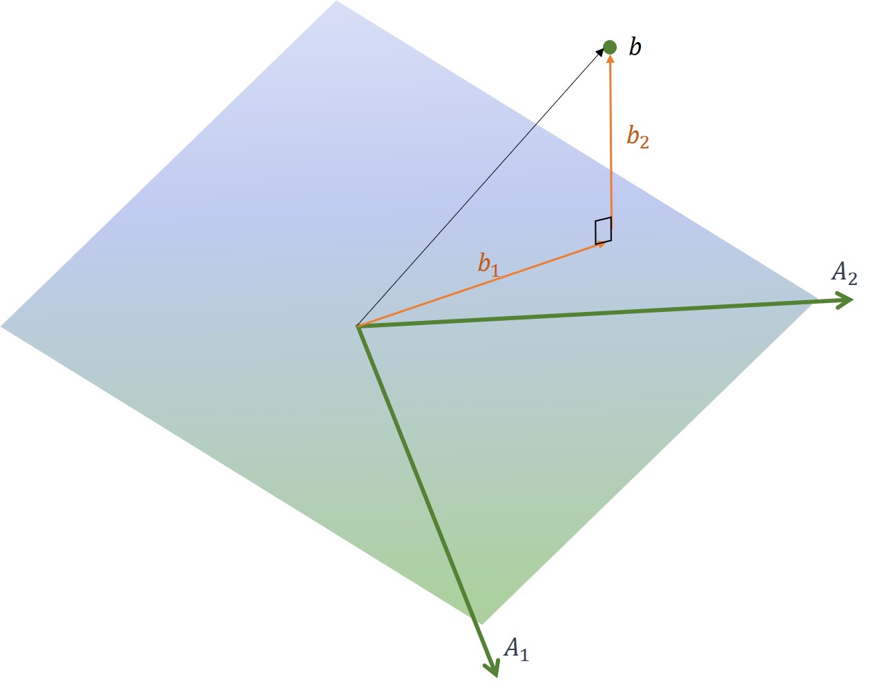
If Ax=b is not feasible, then b lies outside the column space of A, denoted as C(A) (the subspace in Rm spanned by the column vectors of A).
Let N(AT) be the subspace orthogonal to C(A).
We can decompose b into two part:
b=b1+b2,
where b1∈C(A) is in the columns space of A and b2∈N(AT) is orthogonal to the columns space of A.
By assumption we have b2=0.
Suppose y is a feasible solution to yTA=cT.
Then for all k∈R, y+k⋅b2 is still a feasible solution, since
(y+k⋅b2)TA=yTA+k⋅b2TA=yTA=cT.
The new solution has objective
(y+k⋅b2)Tb=yTb+k⋅∥b2∥22.
When k→−∞, we have yTb+k⋅∥b2∥22→−∞, which implies that the primal is unbounded.
General Case
We discuss the more general form:
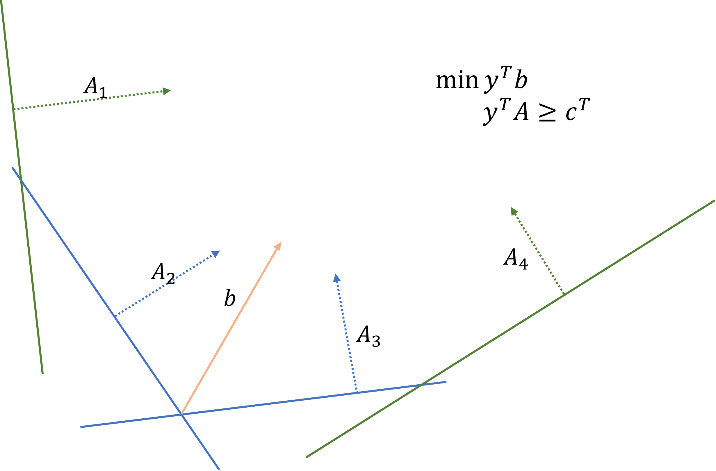
mins.t. yTb,yTA≥cT.
Every linear program can be converted into this general form.
Its dual is given by
maxs.t. cTx,Ax=b,x≥0.
By weak duality,
cTx≤yTAx=yTb
To prove strong duality, we need only to prove that
If both primal and dual are feasible, then there exists feasible x,y, such that cTx=yTAx.
Define the feasible set of the primal as
F≐{y∈Rm:yTA≥cT}.
Let y⋆ be the optimal solution for the primal.
We see that y⋆ can not be an interior point of the feasible set F.
Otherwise, for small enough k>0, y⋆−k⋅b belongs to F.
But (y⋆−k⋅b)Tb<y⋆b, contradicting y⋆ being optimal.
Therefore, y⋆ must be on the boundary of the F, and there must exit one or more constraints saturated by y⋆.
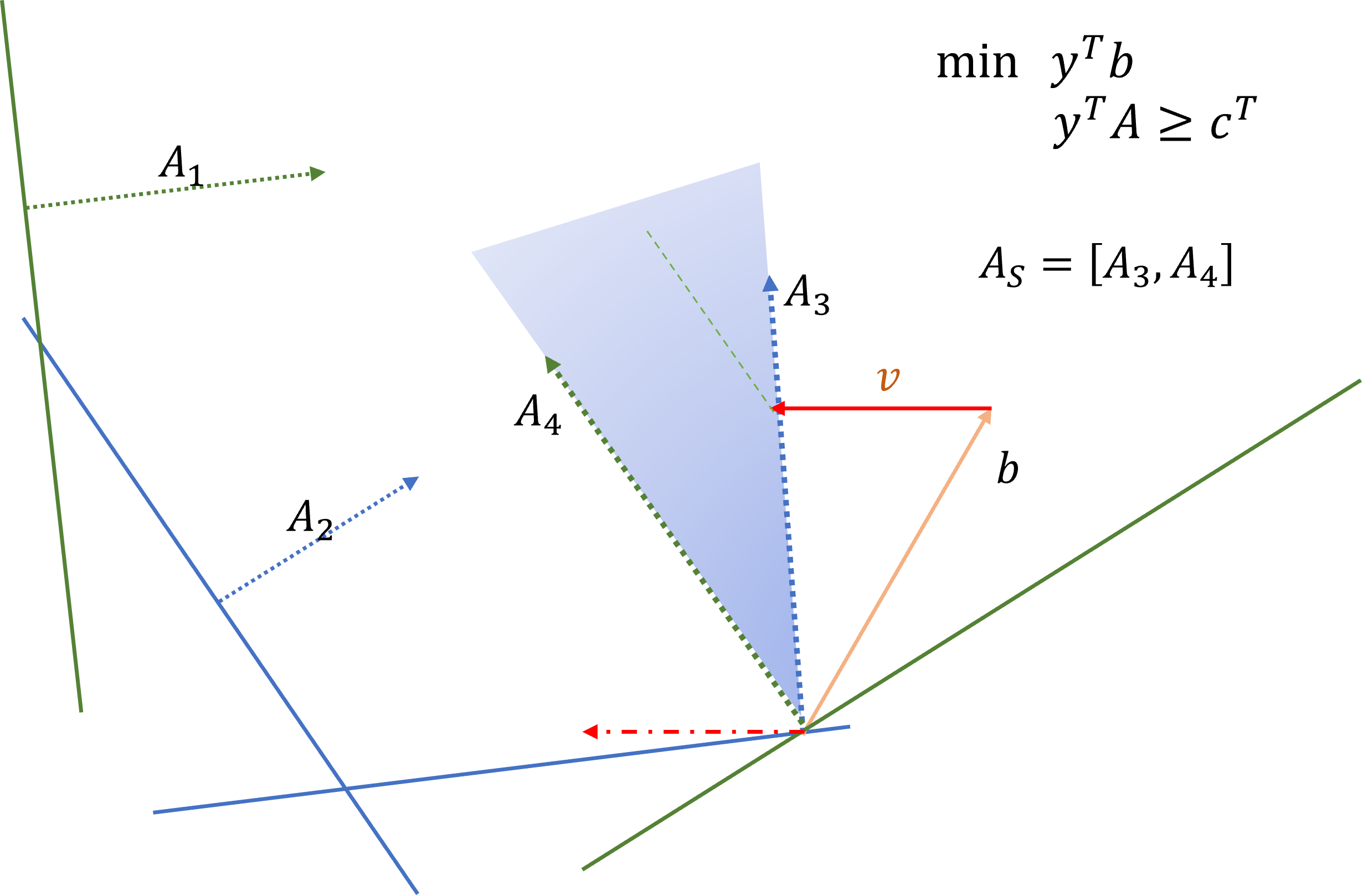
Define the set of indexes of the constraints that are saturated by y⋆
S≐{i∈[m]:(y⋆)TAi=ci}⊆[m],
where Ai is the i-th column of matrix A and ci is the i-th coordinator of vector c.
Let AS be set of columns indexed by S.
Lemma.b is in the conic hull of columns of AS, i.e., ∃xS∈R∣S∣, such that
ASxS=b.
xS≥0.
Such xS can be converted into a feasible solution x to the dual (by padding zeros in dimensions other than S).
It holds that
cTx=(y⋆)TAx=(y⋆)T(ASxS)=(y⋆)Tb.
Question to ponder: prove the existence of optimal solution of the primal, assuming feasibility of the dual.
Proof.
We prove that if b is not in the conic hull of AS, we can more y⋆ along some direction that decreases objective while maintaining feasibility.
By Farkas' Lemma, if b is not in the conic hull of AS, ∃v∈Rm, such that
vTAS≥0.
vTb<0.
Then we can move the vector y⋆ along the direction of v, by adding k⋅v to y⋆ for some k≥0.
This decreases the objective
(y⋆+k⋅v)Tb=(y⋆)Tb+k⋅vTb<(y⋆)Tb.
How large can k be, so the constraints (y⋆+k⋅v)TA≥cT are maintained.