Determinant, Cross Product and Cramer's-Rule

Determinant

When studying linear algebra, the determinant function $\det(\cdot)$ is a horrifying subject. We try to give a friendly approach to it in this article.

I think it is the study of the volume of the parallelotope specified by $v_1, v_2, ... ,v_n \in \mathbb{R}^n$ that gives it away. The parallelotope is defined as the set

\left\{ \sum_{i \in [n]} \lambda_i v_i : \lambda_i \in [0, 1], \forall i \in [n] \right\}

Let's denote $f(v_1, v_2, ... ,v_n) : \mathbb{R}^{n \times n} \rightarrow \mathbb{R}$ the singed volume function, i.e., $|f(v_1, v_2, ... ,v_n)|$ gives the volume of the parallelotope. We will show how to determine the sign of $f$ later. At this point, we do not know how $\det(\cdot)$ is related to the volume. Therefore, we use the notation $f$ instead.

We show how to derive the formula of $f$ by its properties. The two key properties associated with volume are

$f$ is multi-linear. Specially, it is a linear function in any dimension when other dimensions are fixed:
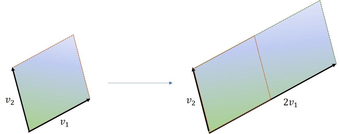
- $f(v_1, v_2, ..., cv_i, ... ,v_n)=cf(v_1, v_2, ... ,v_n)$ for $\forall i \in [n]$ and $c \in \mathbb{R}$ . Geometrically, if we scale the $i$ -th vector $v_i$ by a factor $c$ , then the volume of the parallelotope should change by the same factor. In the above example, when $v_2$ is fixed, the area of the parallelogram is determined by its height, i.e., the projection of $v_1$ to the orthogonal direction of $v_2$ . When $v_1$ doubles, the length of its projection doubles.
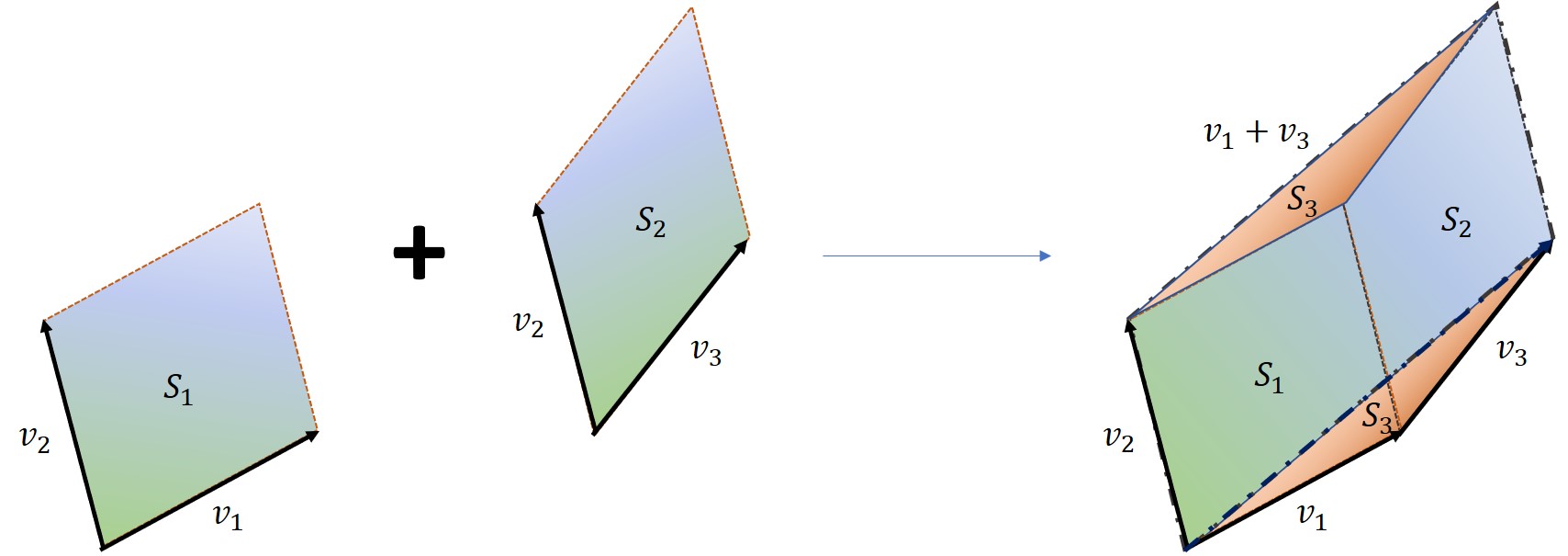
- $f(v_1, v_2, ..., v_i + u_i, ... ,v_n)= f(v_1, v_2, ..., v_i, ... ,v_n) + f(v_1, v_2, ..., u_i, ... ,v_n)$ . In the above example, when $v_2$ is fixed, the projection to the orthogonal direction of $v_2$ are additive. In particular, denote $\mathcal{P}(v_1)$ the length of the projection of $v_1$ to the orthogonal direction of $v_2$ . Similarly we define $\mathcal{P}(v_2)$ and $\mathcal{P}(v_1 + v_2)$ . Then
$\mathcal{P}(v_1 + v_2) = \mathcal{P}(v_1) + \mathcal{P}(v_2)$
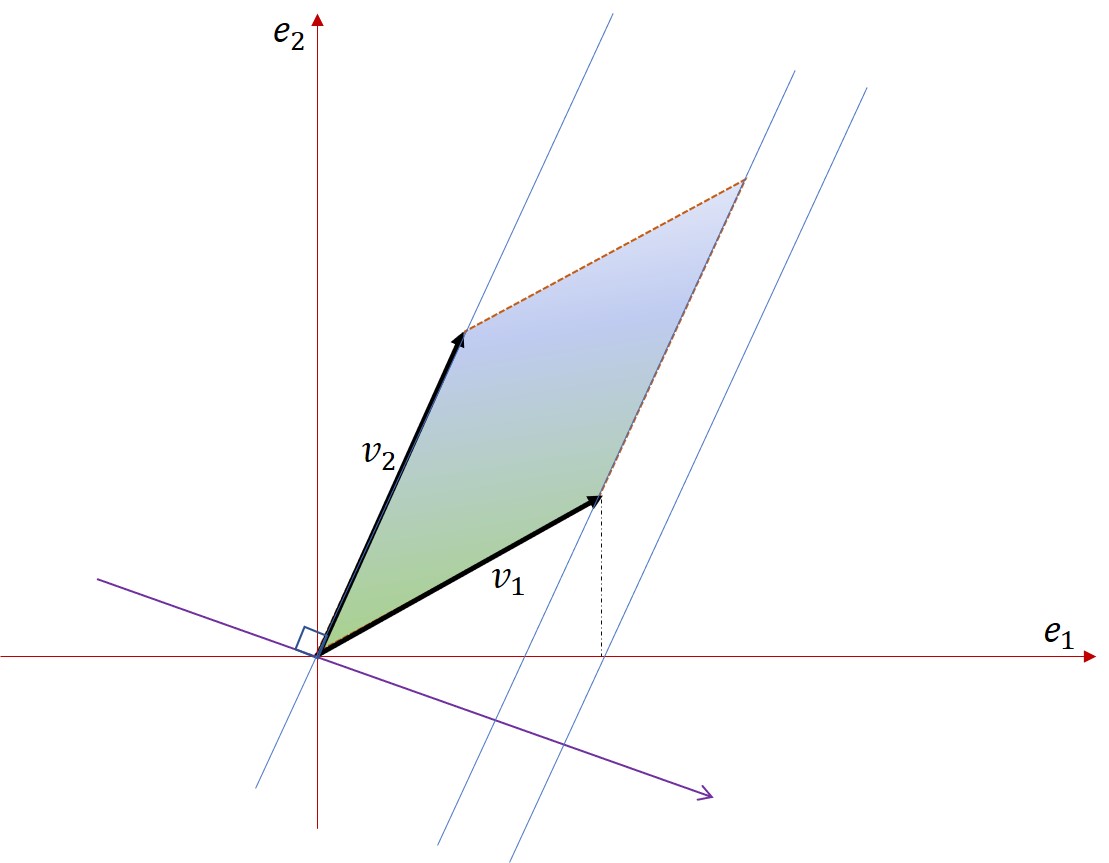
- Note that the projection of two vector can cancel each other in some cases, in the sense that they points to different direction. In the above example, if we write $v_1 = v_{1, 1} e_1 + v_{1, 2} e_2$ , then $\mathcal{P} (v_{1, 1} e_1)$ and $\mathcal{P} (v_{1,2} e_2)$ points to opposite directions. This implies that we should give volume a sign. For example, we can define the direction pointed by purple vector points to be positive. The volume of the parallelogram increases if a vector's projection moves along this direction and decrease otherwise.
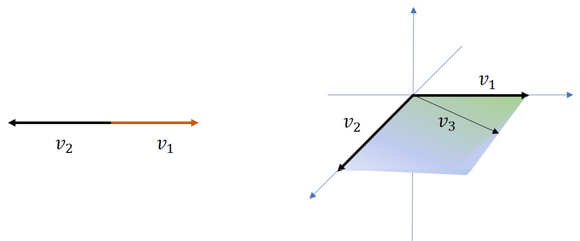
If $v_1, v_2, ..., v_n$ are linearly independent, then the parallelotope is contained in a subspace with dimension smaller than $n$ and should have volume zero. Intuitively, the parallelotope collapses to a lower dimension space. Examples include colinear vectors in two dimension case and the third vector lying in the hyperplane spanned by the other two in the three dimension case.
Finally, we emphases an important case here:

f(..., v_i,..., v_j, ... , ) = 0, \textbf{ if } v_i = v_j, \forall i, j \in [n], i \neq j

If we write

v_i = v_{i, 1} e_1 + v_{i, 2} e_2 + ... + v_{i, n} e_n

for all $i \in [n]$ , then by linearity

\begin{aligned} f(v_1, v_2, ..., v_n) &= f( v_{1, 1} e_1 + v_{1, 2} e_2 + ... + v_{1, n} e_n, \\ &\qquad v_{2, 1} e_1 + v_{2, 2} e_2 + ... + v_{2, n} e_n, \\ &\qquad ...\\ &\qquad v_{n, 1} e_1 + v_{n, 2} e_2 + ... + v_{n, n} e_n) \\ &= \sum_{k_1, k_2, ..., k_n \in [n]} v_{1, k_1} v_{2, k_2} ... v_{n, k_n} f(e_{k_1}, e_{k_2}, ..., e_{k_n}) \end{aligned}

Note that if $k_i = k_j$ for $i \neq j$ , then $f(e_{k_1}, e_{k_2}, ..., e_{k_n}) = 0$ . Therefore,

f(v_1, v_2, ..., v_n) = \sum_{ k \text{ is a permutation} } v_{1, k_1} v_{2, k_2} ... v_{n, k_n} f(e_{k_1}, e_{k_2}, ..., e_{k_n})

We are almost done. It is left to determined the value of $f(e_{k_1}, e_{k_2}, ..., e_{k_n})$ , where $k = (k_1, k_2, ..., k_n)$ is a permutation of $(1, 2, ...., n)$ . Here we claim that is purely determined by the value of $f(e_1, e_2, ..., e_n)$ . By conversion, we define

f(e_1, e_2, ..., e_n) = 1

Then we have the key lemma:

Lemma

f(e_{k_1}, e_{k_2}, ..., e_{k_n}) = -1

if ${k_1}, {k_2}, ..., {k_n}$ can be recovered to $1, 2, ..., n$ by odd number of neighboring swaps and

f(e_{k_1}, e_{k_2}, ..., e_{k_n}) = 1

if ${k_1}, {k_2}, ..., {k_n}$ can be recovered to $1, 2, ..., n$ by even number of neighboring swaps.

Proof. The key is to prove that we swap two neighboring vectors, then the sign of the volume change:

f(e_{k_1}, e_{k_2}, ..., e_{k_{i } }, e_{k_{i + 1} }, ..., e_{k_n}) = -f(e_{k_1}, e_{k_2}, ..., e_{k_{i + 1 } }, e_{k_{i } }, ..., e_{k_n})

This is because

\begin{aligned} f(e_{k_1}, e_{k_2}, ..., e_{k_{i } } + e_{k_{i + 1} }, e_{k_{i } } + e_{k_{i + 1} }, ..., e_{k_n}) &= f(e_{k_1}, e_{k_2}, ..., e_{k_{i } }, e_{k_{i + 1} }, ..., e_{k_n})\\ &\quad + f(e_{k_1}, e_{k_2}, ..., e_{k_{i + 1 } }, e_{k_{i } }, ..., e_{k_n}) \\ &= 0 \end{aligned}

$\square$

Cross Product

If we fix $v_2, v_3, ..., v_n$ , then $\det(x, v_2, ..., v_n): \R^n \rightarrow \R$ is a linear function. Then

\begin{aligned} \det(x, v_2, ..., v_n) &= \sum_{i = 1}^n \det(x_i e_i, v_2, ..., v_n) \\ &= \sum_{i = 1}^n x_i \det(e_i, v_2, ..., v_n) \end{aligned}

where $x_i$ is the i-th coordinator of $x$ . If we write

d = \left< det(e_1, v_2, ..., v_n), det(e_2, v_2, ..., v_n), ..., det(e_n, v_2, ..., v_n)\right>

Then

\det(x, v_2, ..., v_n) = d \cdot x

Indeed, in a similar manner, we can prove that for any $h: \R^{n \times n} \rightarrow \R^n$ linear function, there exists a vector $\vec h$ , such that

h(x) = \vec h \cdot x

Conventionally, $d$ is called the cross product of $v_2, ..., v_n$ is written as

d = v_2 \times v_3 \times ... \times v_n

It has some interesting properties:

$d$ is perpendicular to the subspace spanned by $v_2, ..., v_n$ , as $d \cdot v_i = \det(v_i, v_2, ..., v_n) = 0$ for $2 \le i \le n$ .
For any $x \in \R^n$ , $d \cdot x$ gives the signed volume of the parallelotope spanned by $x, v_2, ..., v_n$ .
- When $n = 2$ , the length of $d$ equals to that of $v_2$ .
- When $n = 3$ , the length of $d$ equals to the area of the parallelogram spanned by $v_2, v_3$ . Combined with the fact that $d$ is perpendicular to $v_2, v_3$ , we see why $d \cdot x$ gives the volume of the parallelotope spanned by $x, v_2, v_3$ : it takes the projection of $x$ to the direction that is perpendicular to $v_2$ and $v_3$ , scaled by a factor of the area spanned by $v_2$ and $v_3$ .
The direction given of $d$ is given by right hand rule, when $n = 2$ or $n = 3$ .

$\square$

Cramer's Rule

Cramer's rule is a formula for solving linear equations. In particular, given an invertible matrix $A \in \R^{n \times n}$ , and vector $b \in \R^n$ , then the solution for the equation

Ax = b

is given by ( $\forall i \in [n]$ ),

x_i = \frac{\det(A_i) }{\det (A)}

where $x_i$ is the i-th coordinate of $x$ and $A_i$ is the matrix formed by replacing $A$ 's the $i$ -th column by column vector $b$ .

To understand the formula, we view $A$ as a mapping $T: \R^n \rightarrow \R^n$ that takes $e_i (i \in [n])$ to $A[:,i]$ , i.e.,

T(e_i) = A[:, i]

where $A[:, i]$ is the i-th column of $A$ . The image of the hypercube

\left\{ \sum_{i \in [n]} \lambda_i e_i : \lambda_i \in [0, 1], \forall i \in [n] \right\}

is given as

\left\{ \sum_{i \in [n]} \lambda_i A[:, i] : \lambda_i \in [0, 1], \forall i \in [n] \right\}

Original the hypercube has volume 1. After the transformation it has volume $\det(A)$ . One interesting fact about linear transformation is that it preserves volumes ratio. Define $\mathbb{V}(\cdot)$ the volume of a parallelotope.

Fact. For any parallelotope $P$ , its volume under transformation $T$ is given by

\det(A) \mathbb{V}(P) = \mathbb{V}(T(P))

Now, we rewrite the Cramer's rule as

\det(A) x_i = \det(A_i)

Its meaning is clear: there is a parallelotope $P$ whose volume is $x_i$ and after the transformation it has volume $\det(A_i)$ .

It is left to verify that the parallelotope indeed exists. We observe that $\det(A_i)$ can be viewed as the volume of the following parallelotope formed by

\left\{ \sum_{j \in [n], j \neq i} \lambda_j A[:, j] +\lambda_i b_i: \lambda_j \in [0, 1], \forall j, \lambda_i \in [0, 1] \right\}

But this parallel0tope is the image of

\left\{ \sum_{j \in [n], j \neq i} \lambda_j e_j +\lambda_i x_i: \lambda_j \in [0, 1], \forall j, \lambda_i \in [0, 1] \right\}

\begin{aligned} & T \left( \left\{ \sum_{j \in [n], j \neq i} \lambda_j e_j +\lambda_i x_i: \lambda_j \in [0, 1], \forall j, \lambda_i \in [0, 1] \right\} \right) \\ &= \left\{ \sum_{j \in [n], j \neq i} \lambda_j T(e_j) +\lambda_i T(x_i): \lambda_j \in [0, 1], \forall j, \lambda_i \in [0, 1] \right\} \\ &= \left\{ \sum_{j \in [n], j \neq i} \lambda_j A[:, j] +\lambda_i b_i: \lambda_j \in [0, 1], \forall j, \lambda_i \in [0, 1] \right\} \end{aligned}

$\square$