Gradient descent is a greedy search method for optimization, whose analysis varies depending on the kind of constraints you place on it.
We study a baby version of the method.
Let f be a twice continuous differentiable and convex function.
We are interested in the minimization problem:
x∈Rnminf(x)
The convexity of f guarantees the existence of a unique minimum value minx∈Rnf(x).
In addition, we assume that f indeed achieves this minimum value at some point, denoted as x∗.
We need this assumption, as in some case, f can never achieve the minimum value.
For example, let f(x)=ex.
f approaches 0 when x→−∞ but never achieves it.
Notations
Before we delve into the details, we need to define some frequently used notations.
The gradient ∇f(x):Rn→Rn is the vector of partial derivatives of f at point x:
∇f(x)=[∂x1∂f(x),∂x2∂f(x),..,∂xn∂f(x)]
The Hessian ∇2f(x):Rn→Rn×n is the matrix of second order derivatives of f at x:∇f(x)=∂x1∂x1∂2f(x),∂x1∂x2∂2f(x),∂x2∂x1∂2f(x),∂x2∂x2∂2f(x),∂xn∂x1∂2f(x),∂xn∂x2∂2f(x),...,∂x1∂xn∂2f(x)...,∂x2∂xn∂2f(x)......,∂xn∂xn∂2f(x)Since f is twice continuous differentiable, the Hessian is symmetric.
Algorithm
The algorithm is itself very simple.
Gradient Descent Require: Initialization point x0∈Rn; Step size: η∈R+; #iterations: T.
For t∈[T]:
xt+1←xt−η⋅∇f(xt).
Below is an example that show how f decreases as the algorithm iterates.
Convergence
To analyze the convergence rate of f, we need additional assumptions.
Here we adopt two strong ones:
Assumptions.
f is β smooth, i.e., ∇f(z)≤βI for ∀z∈Rn.
f is α strongly convex, i.e., ∇f(z)≥αI for ∀z∈Rn.
β upper bounds the largest possible eigenvalue of the Hessian of f at each point in R, and α lower bounds it.
By definition we have β≥α.
Definitions.
For each t∈[T], let Δt≐f(xt)−f(x∗) be the gap between f(xt) and the minimum value f(x∗).
Let κ≐αβ between β and α.
The following theorem characterize the convergence rate of the algorithm:
Theorem (Convergence Rate).If we set η=β1, then it holds that
Δt≤Δ0(1−κ1)t.
By the theorem, given any ϵ>0, the number of iteration t for which Δt≤ϵ is given by
O(κlogϵΔ0).
Proof:
The proof consists of two parts.
β-smoothness and α-convexity play a role in each part separately.
The first claim states that
Claim 1. If η=1/β, then
Δt+1≤Δt−2β1∥∇f(xt)∥2.
We might still have a problem, if when xt approaches x∗, ∥∇f(xt)∥ decreases too fast. That where α convexity comes into play.
Claim 2.
−2α1⋅∥∇f(xt)∥2≤Δt.
In combination, we conclude that
Δt+1≤Δt(1−βα).
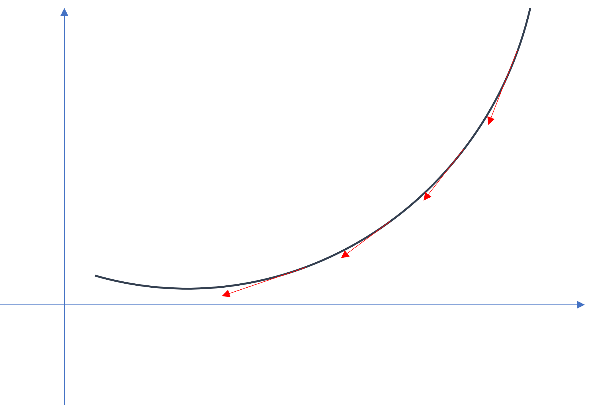
The figure gives some intuition about the algorithm.
The function f is plotted as the blue, real line.
Suppose that A=f(xt).
We search along the direction of −∇f(x) for the minimum value of f(x) by computing xt+1=xt−η∇f(x).
We don't want η to be too large, such that xt+1 passes the minimum point.
How do we guarantee this?
We create a quadratic approximation y=f(xt)+∇f(xt)(y−x)+(β/2)⋅∥y−x∥22 of the f at xt, whose Hessian is βI, which upper bounds the Hessian of f at every point.
The minimum point of the quadratic approximation is a conservative estimate of f(xt).
As we will prove, it holds that
f(x∗)≤f(xt)−2β1∥∇f(xt)∥22.
Proof of the Lemma.
Via Taylor's expansion, for all x,y∈Rn, there exists some z∈[x,y], such that
The figure gives some intuition about the algorithm. The function is plotted as the blue, real line. Suppose that . We search along the direction of for the minimum value of by computing .