Cycle-Core Connection Game

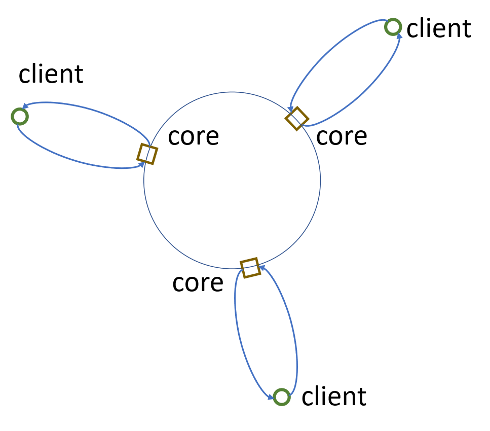
Eisenbrand et al [1] proposed an interesting technique called cycle connection game. In the setting, there is a set of $n$ core points connected by an undirected cycle. Each core point is associated with a client. There is a pair of opposite directed edges between each core point and its associated client. Each edge has a weight. We denote $G$ be the resulting graph.

An example is shown as follows:

Given an instance, we would like to sample a set of clients randomly (we call the sampled clients the "marked" ones). Then each client sends a unit capacity flow to its nearest marked client (could be itself). The cost of each flow is the sum of edges weights it travels. We would like to bound the expected cost of sending the flows.

The selection process requires a probability $p$ as input and consists of two steps:

1. Pick a client uniformly at random. This step ensures that at least one client is selected.
2. For the rest clients, pick each of them independently with some probability $p$.

To analyze the expected cost, we divide the edges into three categories:

1. Directed edges from the clients to the core points, denoted as $\mathcal{E}_{in}$;
2. Directed edges from the core points to the clients, denoted as $\mathcal{E}_{out}$;
3. Edges on the cycle, denoted as $\mathcal{C}$.

The following theorem holds:

Theorem. The expected cost is bounded by

$$\sum_{e \in \mathcal{E}_{in} \cup \mathcal{E}_{out} } w_e + \frac{1}{2p} \sum_{e \in \mathcal{C} } w_e$$

Proof.
For each edge $e$, define a random variable $X_e$ to be the flow value of $e$. For $e \in \mathcal{E}_{in}$, it holds that $X_e \in \{0, 1\}$. However, for $e \in \mathcal{E}_{out} \cup \mathcal{C}$, it is possible that $X_e > 1$. By linearity of expectation,

1. For $e \in \mathcal{E}_{in}$, there is a unit flow on $e$ if only the associated client is not sampled. This happens with probability $(1 - \frac{1}{n})(1 - p)$, where $n$ is the number of clients. Therefore, $\mathbb{E} [X_e \cdot w_e] = (1 - \frac{1}{n})(1 - p) \cdot w_e$ and

   $$\mathbb{E} \left[ \sum_{e \in \mathcal{E}_{in} } X_e \cdot w_e \right] = (1 - \frac{1}{n})(1 - p) \cdot \sum_{ e \in \mathcal{E}_{in} } w_e.$$

2. For $e \in \mathcal{E}_{out}$, the analysis is a little tricky. For each particular sample instance, it holds that $\sum_{e \in \mathcal{E}_{out}} X_e = \sum_{e \in \mathcal{E}_{in}} X_e$, by flow conservation. Therefore,

   $$\mathbb{E} \left[ \sum_{e \in \mathcal{E}_{out}} X_e \right] = \mathbb{E} \left[ \sum_{e \in \mathcal{E}_{in}} X_e \right] = (1 - \frac{1}{n})(1 - p) n.$$

   By symmetry, $\{ X_e \}_{ e \in \mathcal{E}_{out} }$ are identical distributed random variables. Therefore $\mathbb{E} [X_e] = (1 - \frac{1}{n})(1 - p)$. It concludes that

   $$\mathbb{E} \left[ \sum_{e \in \mathcal{E}_{out} } X_e \cdot w_e \right] = (1 - \frac{1}{n})(1 - p) \cdot \sum_{ e \in \mathcal{E}_{out} } w_e.$$

3. For $e \in \mathcal{C}$, the analysis of $\mathbb{E} [X_e]$ is the hardest part. We look at the suboptimal flow routing scheme such that each un-marked client sends a unit flow to a nearest marked client, with respect to unit cycle edge weight. Let $Y_e$ be the number of flows on edge $e$. Clearly,

   $$\mathbb{E} \left[ \sum_{e \in \mathcal{C} } X_e \cdot w_e \right] \le \mathbb{E} \left[ \sum_{e \in \mathcal{C} } Y_e \cdot w_e \right].$$

   Further, for each client $j$, let the random variable $Y_j$ be the number of cycle edges travelled by its flow, then

   $$\sum_{e \in \mathcal{C} } Y_e = \sum_j Y_j.$$

   For a fixed $j$ and some integer $0 \le k \le \lfloor (n - 2) / 2 \rfloor$, the event $Y_j > k$ happens if and only if $j$ is not marked and none of the first $k$ client neighbors to the left and right of $j$ is marked, the probability of which is given by

   $$\Pr[Y_j > k] = \left( 1 - \frac{2k + 1}{n} \right) q^{2k + 1}.$$

   where $q = (1 - p)$. Now the expectation of $Y_j$ is given by

   $$\begin{aligned} \mathbb{E} [Y_j] &= \sum_{k = 0}^{\lfloor (n - 2) / 2 \rfloor } \left( 1 - \frac{2k + 1}{n} \right) q^{2k + 1} \\ &\le e^{ - \frac{ 1 }{n} } q \sum_{k = 0}^{\lfloor (n - 2) / 2 \rfloor } e^{ - k \frac{ 2 }{n} } q^{k2} \\ &\le e^{ - \frac{ 1 }{n} } q \sum_{k = 0}^{\lfloor (n - 2) / 2 \rfloor } (e^{ - \frac{ 2 }{n} } q^{2} )^k \\ &= e^{ - \frac{ 1 }{n} } q \frac{ (1 - (e^{ - \frac{ 2 }{n} } q^{2} )^{\lfloor (n - 2) / 2 \rfloor } ) }{1 - (e^{ - \frac{ 2 }{n} } q^{2} ) } \\ &\le \frac{ e^{ - \frac{ 1 }{n} } q }{ 1 - (e^{ - \frac{ 2 }{n} } q^{2} ) } \\ &\le \frac{1}{ 2 (1 - e^{ - \frac{ 1 }{n} } q) }. \end{aligned}$$

   The final inequality holds as $2x - 2x^2 \le 1 - x^2$. Replacing $q$ with $1 - p$, we have

   $$\mathbb{E} [Y_j] \le \frac{1}{ 2 (1 - e^{ - \frac{ 1 }{n} } (1 - p)) } \le \frac{1}{ 2 (1 - e^{ - \frac{ 1 }{n} } + e^{ - \frac{ 1 }{n} } p) } \le \frac{1}{2p}.$$

   Remark: a more coarse calculation which leads to the same result would be

   $$\mathbb{E} [Y_j] \le \sum_{k = 0}^\infty (1 - p)^{2k + 1} \le \frac{1 - p}{1 - (1 - p)^2 } \le \frac{1}{2p}.$$

   By symmetry, the $Y_j$'s are identical distributed random variables. So are the variable $Y_e$'s for $e \in \mathcal{C}$. It follows

   $$\begin{aligned} \mathbb{E} [Y_e] = \mathbb{E} [Y_j] &\le \frac{1}{2p}. \end{aligned}$$

   and

   $$\begin{aligned} \mathbb{E} \left[ \sum_{e \in \mathcal{C}} Y_e \cdot w_e \right] &\le \frac{1}{2p} \sum_{e \in \mathcal{C}} w_e. \end{aligned}$$

$\blacksquare$

Reference:

1. Eisenbrand, Friedrich, Fabrizio Grandoni, Thomas Rothvoß, and Guido Schäfer. "Approximating connected facility location problems via random facility sampling and core detouring." In Proceeding of Nineteenth annual ACM-SIAM Symposium (SODA'08), no. CONF, pp. 1174-1183. 2008.

2. Eisenbrand, F., Grandoni, F., Rothvoß, T., Schäfer, G., 2010. Connected facility location via random facility sampling and core detouring. Journal of Computer and System Sciences 76, 709–726.