Splay Tree — Hao Wu

Splay Tree [1] is a self-binary search tree that achieves $O(\log n)$ amortized time complexity for each operation. Unlike other balanced binary search trees, it does not require to maintain additional information to keep balance. Further, it has good property that more recently accessed nodes are more easily retrieved and achieves certain optimality even for an unknown sequence of operations.

Basic Operations

The philosophy of splay tree is very simple: just bring the last accessed node $x$ to the root of the tree, via a sequence of rotations. This brings the most recently visited nodes close to the root.

[Remark: For insertion, the last accessed node is the node inserted. For a successful search operation, the last accessed node is the node found. For an unsuccessful search/deletion, it is the predecessor or successor of the search node / deleted node.]

There is more than one way to rotate a node $x$ to the root. For example, the simplest one rotates $x$ with its parent repeatedly until it becomes the root. However, we can easily find counter examples for this naïve approach. The rotations need to be carefully designed and are called splays. At each step the node being splayed is brought up at most 2 levels. It can be divided into three categories.

Call $x$ the node being splayed, $y$ its parent and $z$ its grandparent (if they exist).

Root case: $x$ is the root. Do nothing.

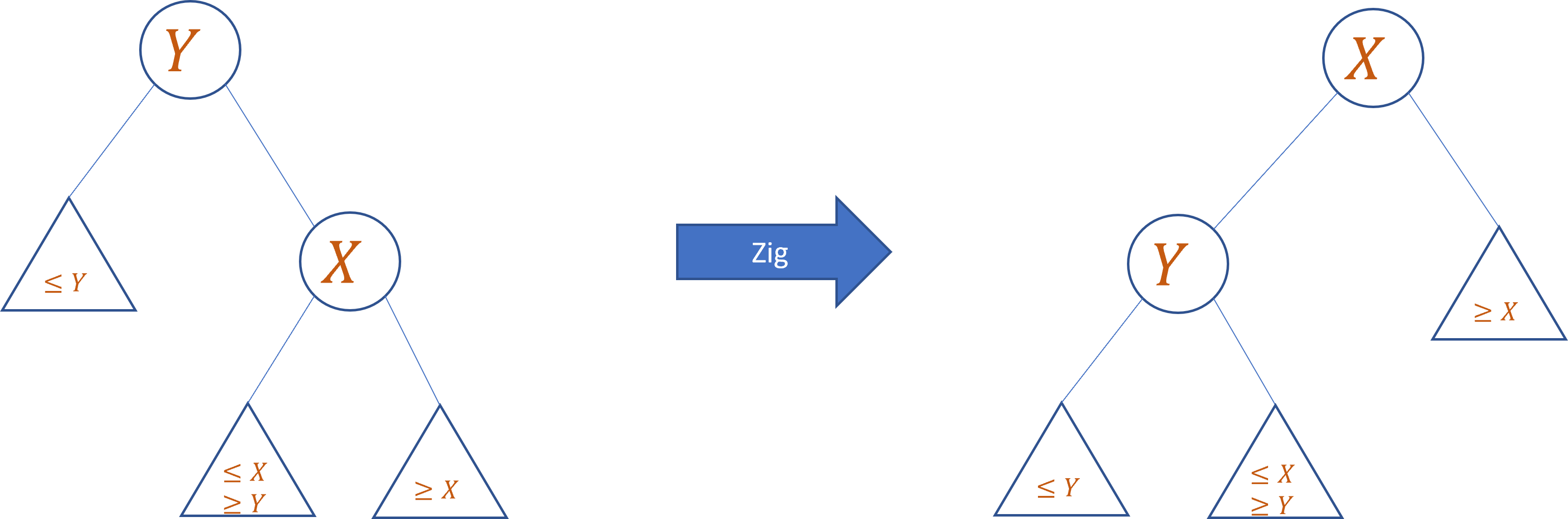
Zig

The Zig case: $y$ is the root. We just perform $rotate(x, y)$ .
- See the following figure.
Otherwise, $x$ has a grandparent $z$ . It is further divided into two categories:

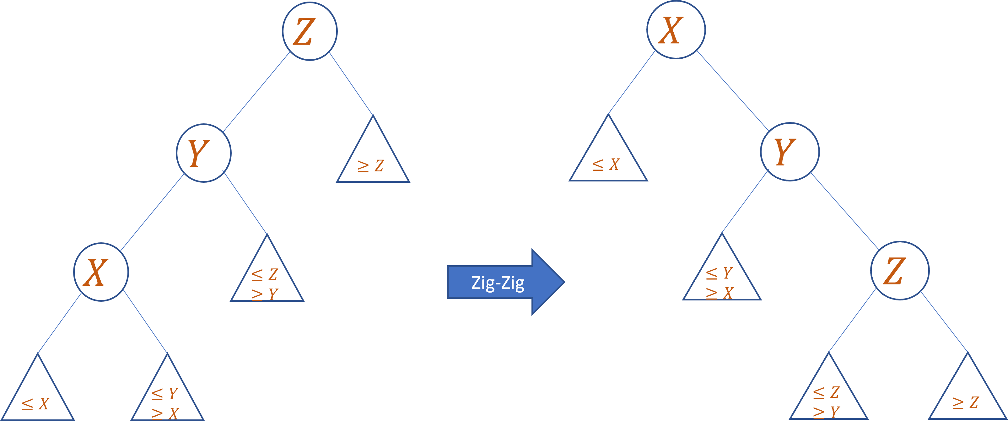
Zig-Zig

Zig-Zig case: both $x$ and $y$ are left children or right children. We first perform $rotate(y, z)$ then $rotate(x, y)$ .

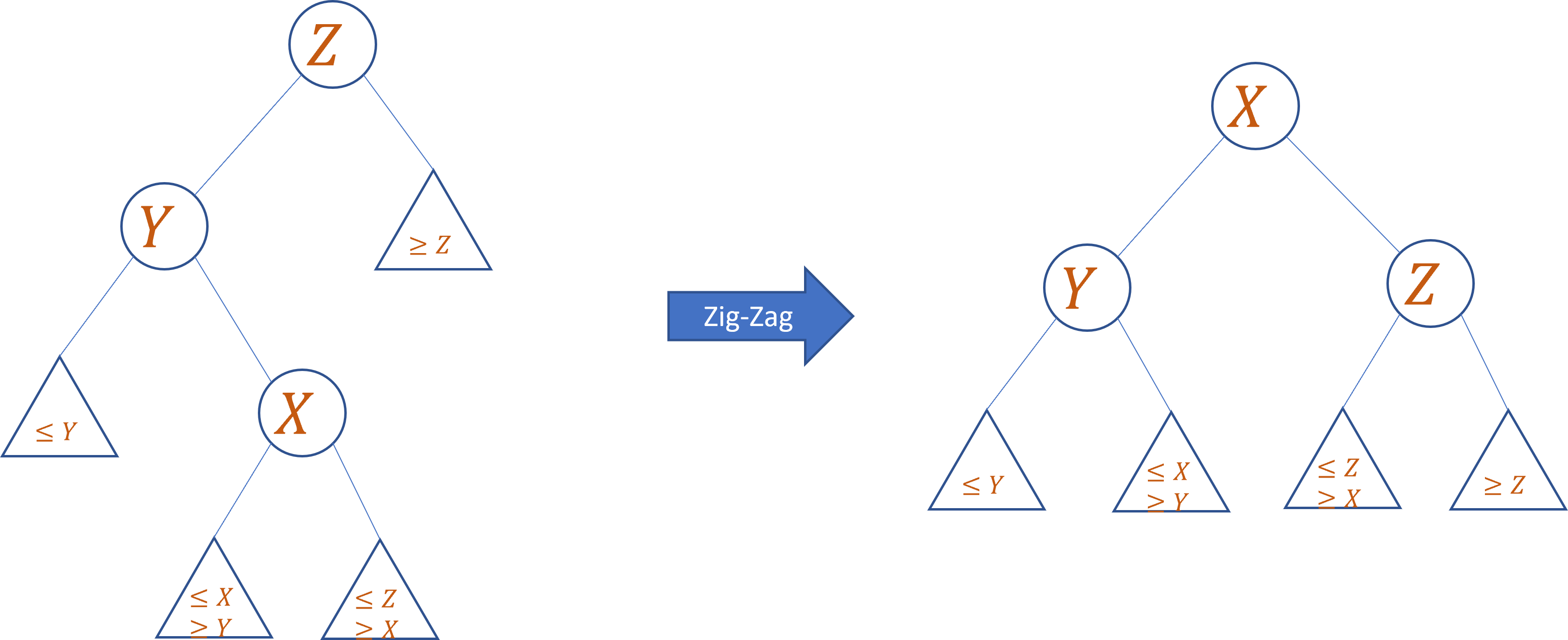
Zig-Zag

Zig-Zag case: $x$ and $y$ are different children of their parents, i.e., $x$ is the left child and $y$ is the right child, or vice versa. We first perform $rotate(x, y)$ then $rotate(y, z)$ .

The splay is performed repeatedly on $x$ until it reaches the root. It is also possible to perform equivalent operations in an top-down approach [1].

Amortized Analysis

There is no explicit control over the height of the tree. It is possible that the accessed node has depth $\Omega(\log n)$ . The intuition is that, however, the imbalanced situation is not easy to create and results from a sequence of previous operations. The number such operations can not be too small to create the imbalance. We can charge the cost of accessing the node with long depth to these previous operations. Intuitively, each such operation is required to reserve some additional "energy" for the amount of imbalanced it creates, which is used later to fix the imbalance. When a long path is encountered, there should be enough "energy" to cover the search on the path, and the subsequent splay costs.

It is left to give a quantitative analysis for keeping the "energy" and for "using" the "energy". We need a few more definitions for a node $x$ .

$T(x):$ the subtree rooted at $x$ .

$w(x):$ the weight associated with node $x$ . This weight is only used for analysis and is not kept explicitly by splay tree.

$s(x)=\sum_{y \in T(x)} w_y:$ the sum of weights of nodes in $T(x)$ , which is referred to as the size of $x$ .

$r(x) \doteq \log s(x)$ , the rank of $x$ .

Let $T$ be the splay tree.

Definition. The potential function, which records the amount of "energy" in $T$ , is defined as
$\Phi(T) = \sum_{x \in T} r(x).$
Definition. The amortized cost of an operation is defined as
$\text{amortized cost} = \text{actual cost} + \Delta \Phi$
where $\Delta \Phi$ is the change of the potential function.

Now, let $r(x)$ be the rank of $x$ before we performed a single splay operation on $x$ and $r'(x)$ the one after. The Access Lemma states the $\Phi$ changes as follows:

Access Lemma For a single splay operation, the potential change is bounded by
$3(r'(x) - r(x)) - 2$
for zig-zig and zig-zag case and
$r'(x) - r(x)$
for the zig case.

Before we prove this key lemma, we use it for the following theorem.

Theorem. The amortized cost of the splaying a node $x$ to the root is
$O \left( 1 + \log \frac{s(root) }{s(x) } \right)$

Proof. To splay a node $x$ to the root, suppose that we have performed $k$ splays. Further, let $r_i(x)$ be the rank of $x$ after we performed the $i^{th}$ splay on $x$ . We have

r_0(x) = \log s(x), \qquad r_k(x) = \log s(root).

Observe that the actual cost of splay operation is $2$ for zig-zig and zig-zag case and 1 for the zig case. Via the access lemma, the amortized cost is

\begin{aligned} \text{amortized cost} &\le \sum_{i \in [k] } 3 \big( r_i(x) - r_{i - 1}(x) \big) +1 \\ &= 3(r_k(x) - r_0(x)) + 1. \end{aligned}

The added 1 results from the final possible zig operation.

$\square$

If we set $w(x) = 1$ for all nodes, then $r_k(x) = \log n$ and $r_1(x) \ge \log 1 = 0$ . Therefore, the amortized cost of splaying $x$ is bounded by $O(\log n)$ .

Proof of The Access Lemma

Zig-Zig

Example.

First,

\begin{aligned} \frac{1}{2} r'(z) + \frac{1}{2} r(x) &= \frac{1}{2} \log s'(z) + \frac{1}{2} \log s(x) \\ &\le \log \left[ \frac{s'(z)}{2} + \frac{ s(x) }{2} \right] \\ &< \log \left[ \frac{s(z)}{2} \right]. \end{aligned}

The first inequality follows from that the function $\log (\cdot )$ is concave and the second one follows from $s'(z) + s(x) = s(z) - 1 < s(z)$ .

Noting that $s(z) = s(x')$ , we have $r(z) = r(x')$ , and

\begin{aligned} & r'(z) + r(x) \le 2 \left[ r(z) - 1 \right] = 2 \left[ r(x') - 1 \right]. \end{aligned}

This implies that

r'(z) \le 2 \left[ r(x') - 1 \right] - r(x).

Now consider the potential change of the zig-zig operation:

\begin{array}{rll} & r'(x) + r'(y) + r'(z) - r(x) - r(y) - r(z) \\ = & r'(y) + r'(z) - r(x) - r(y) \\ \le & r'(x) + r'(z) - 2 r(x) \\ = & r'(x) + \left[ 2 \left[ r(x') - 1 \right] - r(x) \right] - 2 r(x) \\ \le & 3[r'(x) - r(x)] - 2, \end{array}

where the first equality follows from that $r'(x) = r(z)$ , and the first inequality holds since $r(x) \le r(y)$ .

Zig-Zag

Example.

First, note that

\begin{aligned} \frac{1}{2} r'(y) + \frac{1}{2} r'(z) = & \frac{1}{2} \log s'(y) + \frac{1}{2} \log s'(z) \\ \le & \log \left[ \frac{s'(y)}{2} + \frac{ s'(z) }{2} \right] \\ < & \log \left[ \frac{s'(x)}{2} \right]. \end{aligned}

The first inequality follows from that the function $\log (\cdot )$ is concave and the second one follows from $s'(y) + s'(z) = s'(x) - 1 < s'(x)$ .

Therefore,

r'(y) + r'(z) \le 2 \left[ r'(x) - 1 \right]

Now consider the potential change of the zig-zag operation:

\begin{array}{rll} & r'(x) + r'(y) + r'(z) - r(x) - r(y) - r(z) \\ = & r'(y) + r'(z) - r(x) - r(y) \\ \le & r'(y) + r'(z) - 2 r(x) \\ \le & 2 \left[ r'(x) - 1 \right] - 2 r(x) \\ = & 2[r'(x) - r(x)] - 2, \end{array}

where the first equality follows from $r'(x) = r(z)$ , and the first inequality holds since $r(x) \le r(y)$ .

Zig

Example.

Now consider the potential change of the zig-zag operation:

\begin{array}{rll} & r'(x) + r'(y) - r(x) - r(y) \\ = & r'(y) - r(x) \\ \le & r'(x) - r(x) \end{array}

$\square$

Next, we analyze the amortized costs of basic BST operations. Throughout the analysis we assume that $w(x) = 1$ .

Search

Whether the search is successful or not, we splay the last accessed node to the root and charge the cost of going down the tree to the splay-operations. Therefore, the amortized cost is $O(\log n)$ .

Remark: in case of unsuccessful search, we find either the predecessor or successor of the search key.

Insertion

Inserting a node $x$ is the same as that in a BST. Then we splay node $x$ to the root. We charge the cost of going down the tree by the cost of splaying $x$ , which has amortized cost $O(\log n)$ . It is left to analyze the change of $\Phi$ . Let $root = x_1, x_2, ..., x_k, x_{k + 1} = x$ be the root to $x$ path right after inserting $x$ . The insertion of $x$ increases $s(x_1), s(x_2), ..., s(x_{k })$ by 1, therefore,

\begin{aligned} \Delta \Phi &= \sum_{i = 1}^k \log \frac{s(x_i) + 1 }{s(x_i)} \\ &= \log \prod_{i = 1}^k \frac{s(x_i) + 1 }{s(x_i)} \\ &\le \log \frac{s(x_1) + 1}{ s(x_k ) }, \end{aligned}

The last inequality follows from that $s(x_i) \ge s(x_{i + 1}) + 1$ for $i \in [k]$ . Therefore, $\Delta \Phi = O(\log n)$ and the overall amortized cost of insertion is $O(\log n)$ .

Remark: $key(x_{k})$ is either the predecessor or successor of $key(x)$ .

Deletion

As in a BST, deletion is a little bit tricky. Let $x$ be the node to delete and $y$ be its parent (if exists). There are 3 cases

If $x$ is a leaf node, then we just delete it and splay $y$ to the root.
If $x$ has only one child, we replace $x$ with its child as the child of $y$ . Then we delete $x$ and splay $y$ to the root.

The final case uses the first two cases as a sub-routine. We first discuss the amortized cost of the first two cases. The cost of going down to $x$ can be charged to the cost of splaying $y$ to the root, which has amortized cost $O(\log n)$ . Deleting the node decreases the potential function, which will only lower the overall amortized cost. Therefore, the amortized cost of deletion is bounded by $O(\log n)$ .

If $x$ has two children, we find the predecessor node $pred(x)$ of $x$ , which is the node with largest key in $x$ 's left sub-tree. Note that $pred(x)$ has at most one child. Then we delete the node $pred(x)$ . This reduces to case 1 or case 2. Finally we replace the $key(x)$ with $key(pred(x))$ .

Static Optimality

Let $S$ be a sequence of $m$ operations, consists only of successful searches. Let $p_i > 0$ be the number of times the $i^{th}$ element is accessed. Define a static binary search tree to be the one whose structure is fixed. In particular, it can not perform rotations.

Theorem (Static Optimality). The total cost of $S$ performed on the splay tree is at most a constant times the minimum possible cost of $S$ performed a static binary search tree, plus $O(m)$ .

Proof.
Let

$T^*$ be the static binary search tree that minimizes the cost of $S$ .
$d_i$ the depth of the $i^{th}$ element in $T^*$ , i.e. the number of nodes on the path from the root to the $i^{th}$ element. In particular $l(root\, element) = 1$ .

The total search cost of $S$ on $T^*$ is

\sum_{ i \in [n] } p_i \cdot m \cdot d_i.

We are going to prove that the cost for splay tree is

O \left( m + \sum_{ i \in [n] } p_i \cdot m \cdot d_i \right).

To investigate the time for splay tree, we choose a different weight than earlier and just set $w_i = 3^{-d_i}$ . Note that for each $k \in \mathbb{N}^+$ , there can be at most $2^k$ elements with depth $k$ . Hence the sum of weights is bounded by

\sum_{i \in [n]} w_i = \sum_{i \in [n]} \frac{1}{3^{d_i}} \le \sum_{k \ge 1} 2^k \cdot \frac{1}{3^k} \in O(1).

It follows that

s(root) = \log \sum_{i \in [n]} w_i \in O(1).

Further, for each $i \in [n]$ , since $s(i) \ge w_i$ , via the access lemma, the amortized cost of accessing $i^{th}$ element is bounded by

O \left(1 + \log_2 \frac{s(root)}{s(i)} \right) \subset O \left(1 + \log_2 \frac{1}{w_i} \right) = O \left(1 + d_i \right)

For each $k \in [m]$ , let $c_k$ be the actual cost of the $k^{th}$ operation in $S$ and $a_k$ be the amortized cost. Further, let $\Phi_k$ be the potential of the splay tree after the $k^{th}$ operation. Then

\sum_{ k \in [m] } a_k = \sum_{ k \in [m] } \big( c_k + \Phi_k - \Phi_{k - 1} \big) = \Phi_m - \Phi_0 + \sum_{ k \in [m] } c_k.

Hence, the actual cost on this sequence is bounded by

\begin{aligned} \sum_{ k \in [m] } c_k &= \Phi_0 - \Phi_m + \sum_{ k \in [m] } a_k \\ &\in O \left( \Phi_0 - \Phi_m + \sum_{ i \in [n] } p_i \cdot m \cdot \big( 1 + d_i \big) \right) \\ &= O \left( \Phi_0 - \Phi_m + \sum_{ i \in [n] } p_i \cdot m \cdot (d_i + 1) \right) \\ &= O \left( m + \Phi_0 - \Phi_m + \sum_{ i \in [n] } p_i \cdot m \cdot d_i \right) \end{aligned}

It is left to bound $\Phi_0 - \Phi_m$ . Let $r^0(i)$ be the rank of $i^{th}$ before and $r^m(i)$ be the rank after the operations. It holds that $r^0(i) \le r(root) \in O(1)$ , and $r^m(i) \ge \log_2 w(i)$ . Now,

\begin{aligned} \Phi_0 - \Phi_m = \sum_{i \in [n]} \left( r^0(i) - r^m(i) \right) &\in O \left( \sum_{ i \in [n] } \log 3^{d_i} \right) = O \left( \sum_{i \in [n]} d_i \right). \end{aligned}

Under the assumption that each item is accessed at least once, we know $p_i \cdot m \ge 1$ and

\Phi_0 - \Phi_m \in O \left( \sum_{ i \in [n] } p_i \cdot m \cdot d_i \right).

Remark. Of course, we could bound

\sum_{ i \in [n] } d_i \log 3 \le (1 + 2 \cdot 2 + 3 \cdot 2^2 + 4 \cdot 2^3 + ... + (\lfloor \log_2 n \rfloor + 1) \cdot 2^{ \lfloor \log_2 n \rfloor }) \log 3.

Let $\Sigma=1 + 2 \cdot 2 + 3 \cdot 2^2 + 4 \cdot 2^3 + ... + (\lfloor \log_2 n \rfloor + 1) \cdot 2^{ \lfloor \log_2 n \rfloor }$ , then

2 \cdot \Sigma - \Sigma = (\lfloor \log_2 n \rfloor + 1) \cdot 2^{ \lfloor \log_2 n \rfloor + 1} - \sum_{i = 0}^{\lfloor \log_2 n \rfloor - 1} 2^i \in O(n \log n)

Note that $n \log n$ is a lower bound of the access cost of the optimal static binary search tree, under the assumption that each item is accessed at least once.

Remark:

In general,

\sum_{i = 0}^k x^i = \frac{x^{k + 1} - 1}{x - 1}

Applying $x \cdot \frac{\partial}{\partial x}$ to both sides,

\begin{aligned} \sum_{i = 1}^k i x^{i} &= x \cdot \frac{(k + 1) x^k (x - 1) - (x^{k + 1} - 1)}{(x - 1)^2} \\ &= x \cdot \frac{(k + 1) (x^{k +1} - x^k) - (x^{k + 1} - 1)}{(x - 1)^2} \\ &= x \cdot \frac{ k x^{k +1} - (k + 1) x^k + 1}{(x - 1)^2} \\ &= x \cdot \left( \frac{k x^k }{x - 1} - \frac{ x^k - 1}{(x - 1)^2} \right)\\ \end{aligned}

Working Set Property

Suppose that $S = \{x_1, x_2, ..., x_m\}$ and let $t(k)$ be the number of different nodes accessed before $x_k$ since the last access of node $x_k$ , or since the beginning of the sequence if $x_k$ is the first access.

Theorem. The overall cost of $S$ on the splay tree is bounded by
$O \left( m + n \cdot \log n + \sum_{k = 1}^n \log t(k) \right)$

Proof. We maintain $w(x) = \frac{1}{(j + 1)^2}$ , if the sequence accesses $j$ different nodes since the last accessed of node $x$ , or $w(x) = \frac{1}{n^2}$ if it is never accessed before. By definition of $t(k)$ , we have $w(x_k) = \frac{1}{(t(x_k) + 1)^2}$ . Now

W \doteq \sum_{x \in T}^n w(x) \in O(1)

For a node $x_k$ , if it is accessed for the first time, the amortized cost is

O \left( 1 + \log \frac{W}{w(x_k)} \right) = O(\log n) = O(\log t(k))

Summing over all nodes $x$ in the splay tree $T$ , we get $O(n \log n)$ .

Otherwise, if an item $x_k$ is accessed before, the amortized cost of accessing $x_k$ is

O\left( 1 + \log \frac{W}{w(x_k) } \right) = O \left( 1 + \log t(k) \right)

After each access of a node $x_k$ and splaying it to the root, we modify the weights of the nodes as follows: for all node $x$ with $t(x) < t(x_k)$ (the nodes accessed after the last access of $x_k$ ), we set

w(x) = \frac{1}{(t(x) + 1)^2}

This guarantees that $w(x_k) = {1} / {(1 + t(k))^2}$ for $k \in [m]$ .

The weight of the root does not change but the weight of other nodes may decrease after the reassignment. Therefore, the overall potential decreases. The amortized cost of the this access only decreases and is still bounded by $O(1 + \log t(k))$ .

Hence

\sum_{ k \in [m] } a_k \in O \left( n \log n + m + \sum_{ k \in [m] } \log t(k) \right).

Finally, it is easy to see that $\Phi_0 - \Phi_m \in O(n \log n)$ . Therefore,

\sum_{ k \in [m] } c_k \in O \left( n \log n + m + \sum_{ k \in [m] } \log t(k) \right).

$\square$

Static Finger Property

The static finger property states that splay tree achieves some kind of locality. Suppose we order the nodes in the tree in increasing order according to their keys and labels them as $1, 2, ..., n$ . For a node $x$ , we use $\pi(x)$ to denote its order.

Theorem. For any fixed $i \in [n]$ , the total cost of $S$ on the splay tree is bounded by
$O \left( n \log n + m + \sum_{ k \in [m] } \log (|\pi(x_k) - i| + 1) \right).$

Proof. For $x \in T$ , we set $w(x) = \frac{1}{(|pi(x) - i| + 1)^2}$ . Then

W \doteq \sum_{x \in T} \in O(1)

and the amortized cost of accessing $x_k$ is

O \left( 1 + \log \frac{W}{w(x_k)} \right) = O(1 + \log (|\pi(x_k) - i| + 1))

The theorem then follows from $\Phi_0 - \Phi_m = O(n \log n)$ .

$\square$

Reference

[1]. Sleator, D.D. and Tarjan, R.E., 1983. A data structure for dynamic trees. Journal of computer and system sciences, 26(3), pp.362-391.

[2]. Jelani Nelson, Lecture 7, CS 224: Advanced Algorithms.