Integer Shortest Path

Single source shortest path is one of most popular the topics taught in a introductory algorithm course. Given a graph $G = \left< V, E \right>$ with $n$ vertices and $m$ edges, the famous Dijkstra's algorithm has runtime $O(m \log n)$ by using a binary heap. When more advanced heap such such Fibonacci heap is deployed, the runtime can be improved to $O(m + n \log n)$. Most introductory courses are satisfied with the above solutions without going further.

Here we explore the topic by considering a special case where all edge weights are non-negative integers within the set $\{0, 1, 2, ..., C\}$. We develop new heaps incrementally and we will finally see that Dijkstra algorithm can do substantially better than $O(m + n \log n)$.

Time: $O(m + nC)$, Space: $O(nC)$.

As a warm up, we demonstrate an algorithm with runtime $O(m + nC)$ and space overhead $O(nC)$. Here we exclude the space $O(m + n)$ required for storing the graph to simplify the discussion and comparison between the algorithms.

The idea is very simple. We know that the possible distance from any vertex to the source vertex (denoted as $s$) is no less than $nC$. It suffices to keep an array $A_1$ with length $nC$, such that $A_1[i]$ maintains the set of vertices with temporary distance $i$. In this context, we call $A_1[i]$ a bucket and the array $A_1$ itself the buckets.

Initially all $A_1[i]$'s are empty except that $A_1[0]$ contains the source vertex. The algorithm iterates over $A_1$ to find an unmarked vertex with the minimum distance, marked it, update its neighbors' distances and move them to the corresponding buckets.

Each vertex is inserted into $A_1$ once. There are at most $m$ updates of vertices' distances. As the minimum distance of the unmarked vertices is monotonically increasing, we scan the array $A_1$ only once. Summing over the cost we get the $O(m + nC)$ time complexity bound.

Time: $O(m + nC)$, Space: $O(C)$.

The space usage of the above algorithm can be improve to $O(C)$. Relabel the vertices as $s = v_0, v_1, v_2, ..., v_n$ according to the order they are marked.

Suppose that Dijkstra's algorithm uses an array $d$ to record the vertices' distances to $s$. Initially, $d(s) = 0$ and $d(v) = \infty$ for $\forall v \neq s$. Now, consider the moment that $k$ ($0 \le k < n$) vertices have been marked. For $i > k$, the value of $d(v_i)$ is either

1. $d(v_i) = \infty$, if $v_i$ is not adjacent to any vertex $v_j$ for $j \le k$. In this case $v_i$ is not in the array $A_1$.

2. $d(v_i) = d(v_j) + w_{i,j}$ for some $j \le k$, where $w_{i,j}$ is the edge weight between $v_i$ and $v_j$.

By the property of Dijkstra's algorithm, at this moment it also holds that

Therefore, for $i > k$, either $v_i$ is not in $A_1$ or

All un-marked vertices that are in $A_1$ must be in the range of

In general, let $\mu$ be the distance of the least marked vertex. It suffices to maintain a window of $A_1[\mu...\mu+C]$. We can implement this by initializing $A_1$ with size $C+1$ and use it in a wrap-around manner.

Time: $O(m + n \sqrt C)$, Space: $O(C)$.

In previous section, we successfully reduce the size of $A_1$ to $1 + C$. But the runtime remains $O(m + nC)$. To motivate the algorithm discussed in this section, we first provide an alternative view of this complexity:

1. We update the vertices' distance and move the vertices between buckets, which has cost $O(m)$;

2. At each iteration of Dijkstra's algorithm, in the worst case, we need to scan the entire array of $A_1$ to find an unmarked vertex with minimum distance, which takes $O(C)$ times. This is repeated $n$ times.

Where could we have wasted our time? Do we really have spend $O(C)$ time to find the unmarked vertex with minimum distance?

We can improve this to $O(\sqrt C)$ by using two-level buckets. We break the buckets in $A_1$ into $\sqrt { C + 1}$ blocks, each of size $\sqrt { C + 1}$ (assume here $\sqrt { C + 1}$ is an integer for simplicity). For each block, we use one flag bit to indicate whether this block is empty. This results in $\sqrt { C + 1}$ flags bits, which are stored in bit array $A_2$. From now on,

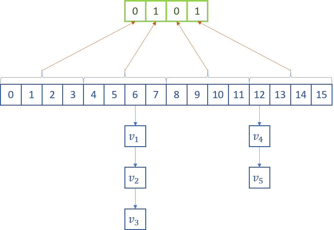
Now, to find an unmarked vertex with minimum distance, we scan $A_2$ to find the first non-zero bit then the corresponding bucket in $A_1$, which takes $O(\sqrt C)$ time. Totaling the runtime, we obtain a bound of $O(m + n \sqrt C)$.

Question to ponder: calculate the size of $\sqrt C$ for some values of $C$ which you consider reasonable in real applications.

Time: $O( m \log_{ \frac{m}{n} } C)$, Space: $O(C)$.

It is natural to extend the idea to $3$-level buckets. Suppose the block size if $\Delta$. Then the third level contains a single bit block of size $\Delta$, the second level contains $\Delta$ bit blocks (with total size $\Delta^3$), and the first level contains the buckets $A_1$ of size $\Delta^3 = C + 1$. It follows that $\Delta = (C + 1)^\frac{1}{3}$ and the time complexity is $O(m + n C^\frac{1}{3} )$.

We may use four level buckets, in which $\Delta = (C + 1)^\frac{1}{4}$ and the time complexity is $O(m + n C^\frac{1}{4})$.

Question to ponder: calculate the size of $C^\frac{1}{3}$ and $C^\frac{1}{4}$ for some values of $C$ which you consider reasonable in real applications.

Does the analysis carry for $k$-level buckets for general value of $k$? No. We can no longer consider the $k$ as a constant and have to take into consider the overhead of insertion, decrease-key and deletion explicitly.

For a $k$-level bucket structure with bucket size $\Delta = (1 + C)^\frac{1}{k} \ge 2$,

1. insertion takes $O(k)$ time,

2. decrease-key takes $O(k)$ time,

as we need to maintain the indicators bits in $2...k$ levels. Finally,

3. delete-min takes $O(k \Delta)$ time,

as we need to scan $k$ buckets, each of size $\Delta$, to find the min element and delete it.

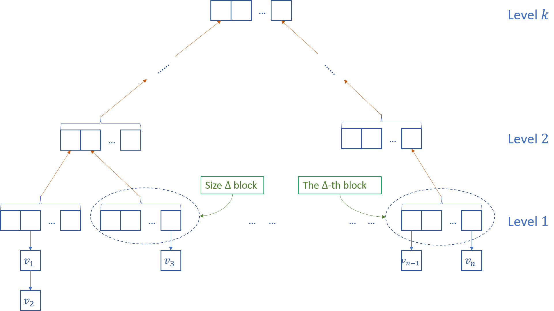
The time complexity now becomes

Balancing the two terms, we get $\frac{1}{k} = \frac{ \log \frac{m}{n} }{ \log C}$, i.e., $k = \log_{\frac{m}{n} } C$. To summarize, the time is

and the space overhead is

Question to ponder: calculate the size of $\log_{\frac{m}{n} } C$ for some values of $C$ which you consider reasonable in real applications.

Time: $O(m + n \frac{\log C}{\log \log C})$, Space: $O( (\frac{\log C}{\log \log C} )^2 )$.

The core idea underlying the k-level bucket structure discussed in the previous section is that every integer $w$ in $[0, C]$ can be written as a base-$\Delta$ number with length at most $k$:

where $w_i \in [0, \Delta)$. For convenience, we write it as

Now the meaning of the $k$-level buckets is clear. The $k^{th}$ level partitions the $w$'s according to the value of $w_{k - 1}$. The $(k - 1)^{th}$ level further partitions the $w$'s according to the value of $w_{k - 2}$, and so on. The path from the top level to bottom level is uniquely determined by the sequence $(w_{k - 1}, w_{k - 2}, ..., w_0)_\Delta$. Indeed, this is a special case of trie, which has alphabet size $\Delta$ and contains only sequence of length $k$.

But we may still waste some work. Remember that our goal for designing the data structure is to find the min element. Therefore, it suffices to distinguish the min element from the rest. We should not waste our effort in determining the relative order between the non-min elements.

In the following example, the min elements $v_1, v_2$ fall into the subtree of the first bucket on the $k^{th}$ level while $v_{n - 1}, v_n$ fall into the last one. As $v_{n - 1}, v_n$ are not min elements, it is unnecessary to maintain a subtree to separate them. Worse still, if later decrease-key is applied to either $v_{n -1}$ or $v_n$, and if the new key has to be moved to a new bucket in the $k^{th}$ level, the effort we have spent in constructing the sub-tree is completely useless.

Instead, we can create an auxiliary set to the last bucket on level $k$, to pus $v_{n - 1}, v_n$ into the set directly. Similar idea apply to $v_3$ in the example.

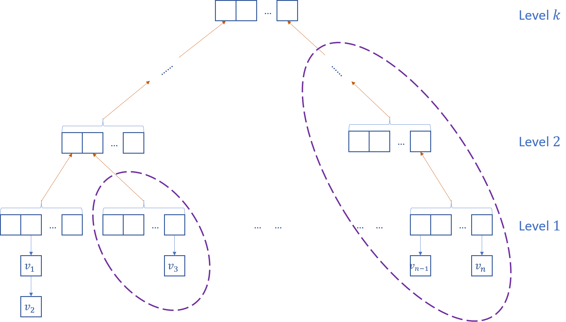
The new structure we get is as follows:

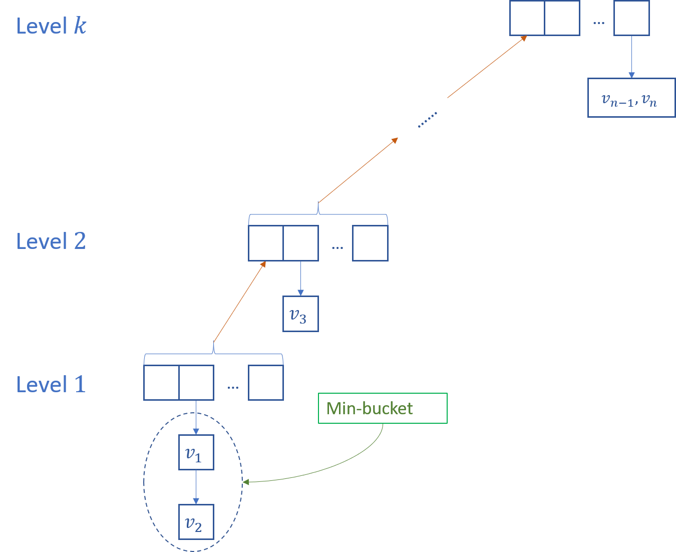
In general, we may not even has a $k$-level trie. In the example below, we can already determine the min-element $v_1$ at some level $i > 1$. Why should we bother to expand the buckets further? Note that this idea is similar to that of trie compression used in Patricia trie.

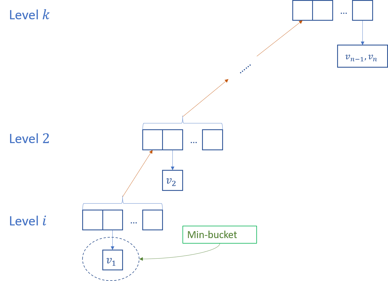
We can be even more lazy. We expand a bucket only when it is necessary. See the example below as an example. In this example, $C = 15$ and $\Delta = 4$.

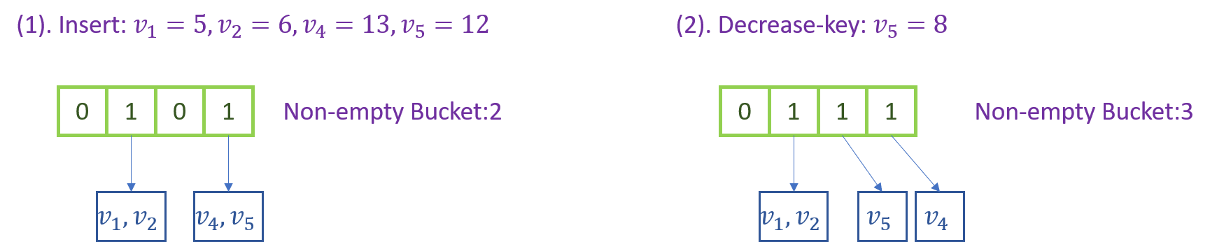
Now, to delete-min, we need to determine the order of $v_1, v_2$.

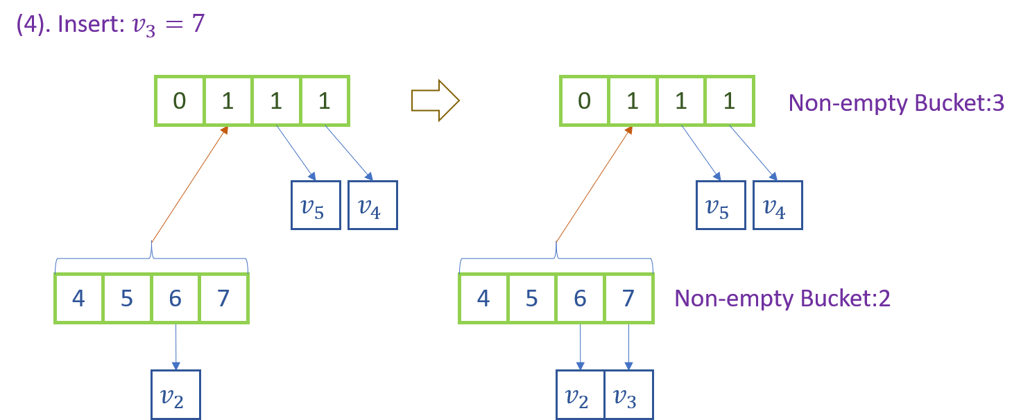
Inserting a new element follows the current structure, until it finds a bucket to fall in.

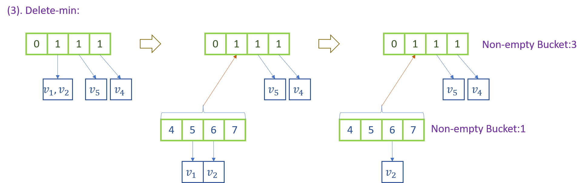
Delete-min begin the search from the lowest level non-empty bucket block.

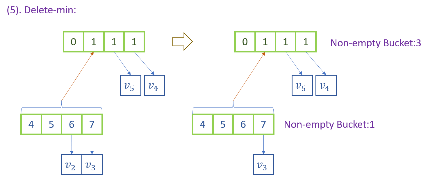
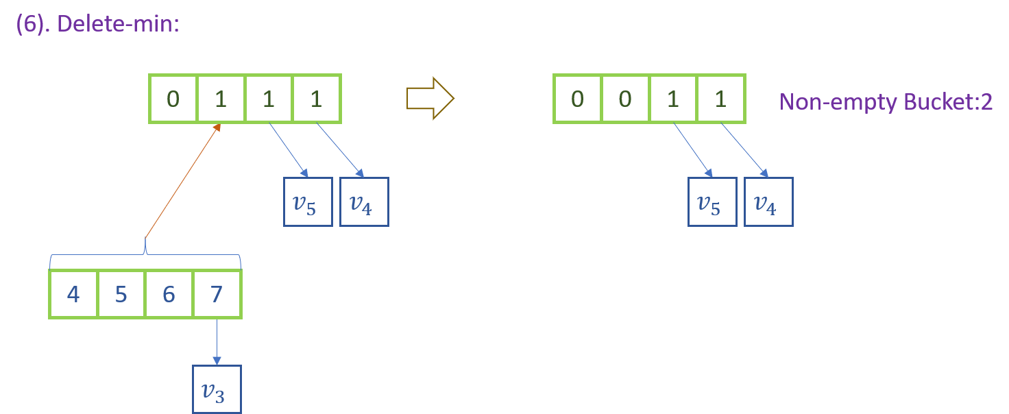
After delete-min, we may need to delete the empty bucket blocks recursively. For each bucket block, we maintain counter for the number of non-empty buckets. This allows us to delete empty bucket blocks in $O(k)$ time.

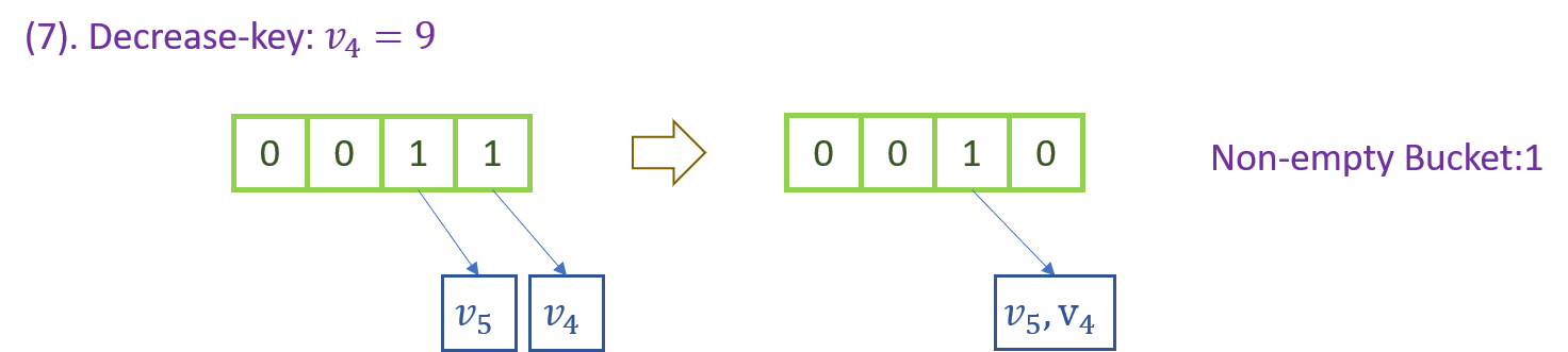
We decrease the key of $v_4$ to 9. Note that we do not need to compare $v_4$ and $v_5$ for the moment. Bucket block counter is maintained when $v_4$ is moved to another bucket.

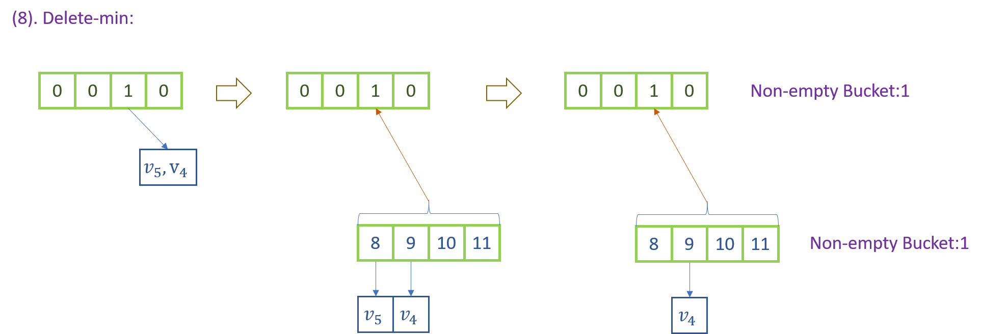
Delete-min is invoked again. We need to expand the bucket containing $v_5$ and $v_4$ to distinguish them.

We continue to insert a new element $v_6 = 12$.

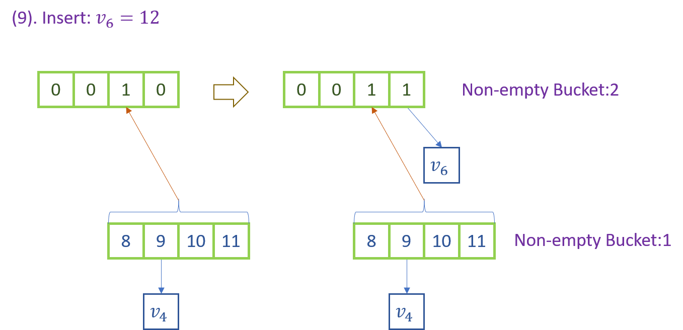
We decrease the key of $v_6$ to $10$. It is pushed down by one level.

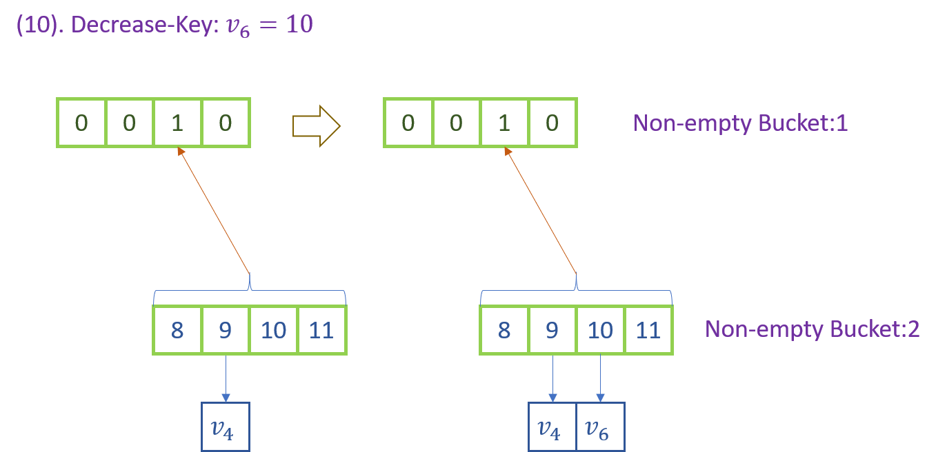
We are now prepared to analyze the amortized cost of these operations:

1. Insert: we pay an $O(k)$ amortized cost of insertion. Any subsequent pushed down operation on this element is charged to its insertion. Note that an element can be push-down by at most $k$ levels.

2. Decrease-key: we pay an $O(1)$ amortized cost of decrease-key operation. The push-down operation is charged to its insertion.

3. Delete-min: to find the min-element, we scan the bucket block in the lowest level to find the first non-empty bucket. This has time $\Delta$. If the bucket found contains multiple elements, we perform an expansion and push the elements down, the cost of which is charged to insertion of these elements. Finally, we may need to delete empty bucket blocks recursively, which has cost $O(k)$.

Therefore, the Dijkstra's algorithm with this structure has runtime $O(m + n(k + \Delta))$, which is minimized when

Solving the equation gives $k = O(\frac{\log C}{\log \log C} )$.

Time: $O( m + n \sqrt{\log C} )$, Space: $O(\sqrt{\log C} \cdot 2^{\sqrt{\log C} })$.

Beginning from the naïve approach, we have improved a lot on both time and space overhead. Amazingly, this is not the end of the story. To motivate what is possibly the inefficient part of $O(m + n \frac{\log C}{\log \log C})$ approach, look at the following example.

Suppose that $C$ is a large number. Initially the structure is empty. We insert an element $v_1$ followed by $v_2$ and they fall into the same bucket in the $k^{th}$ level. Next, we perform a delete-min operation. To distinguish, we expand the buckets all the way down to $1^{st}$ level.

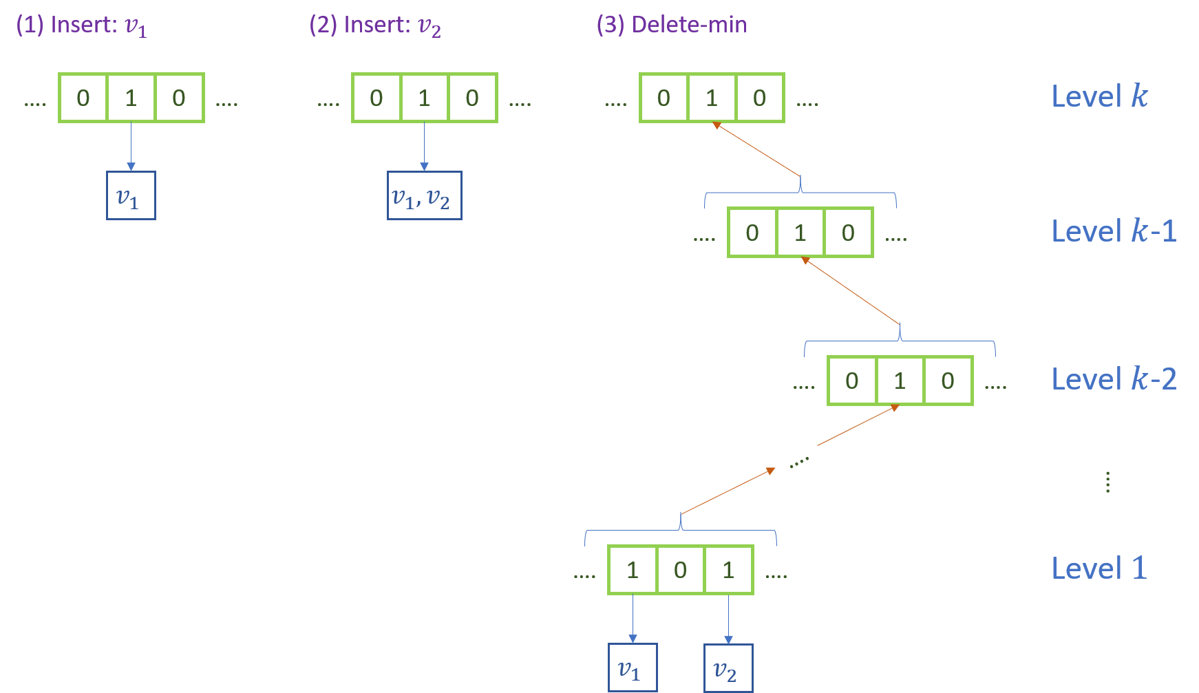
But since there are two elements, why don't we compare them directly and return the minimum one? In such case we avoid the unnecessary expansions.

We can extend the idea further. If the number of elements in a bucket is too few, we refuse to expand it. Instead we make of copy of the elements and construct a comparison based priority queue (e.g., Fibonacci heap) on them. Further, note that we are only interested in the possible min-element. Therefore the heap is constructed for only one bucket that contains the min-element.

We use a parameter $t$ (to be determined) to control this number. In particular, if the number is at most $t$, we construct a comparison based priority queue. We perform expansion only if the number exceeds $t$.

1. Insert: insert an element as before. If the element falls into the bucket that is associated with a priority, then also insert this element into the heap.

2. Decrease-key: if the element is in the bucket that is associated with a priority queue, perform decrease-key in the queue. Otherwise, perform decrease-key as before. If the element falls into the bucket that is associated with a priority queue, then also insert this element into the heap.

3. Delete-min:

1. Find the first non-empty bucket in the lowest level
2. IF the bucket has more than $t$ elements THEN
3. $\qquad$ Expand the bucket
4. $\qquad$ GO TO STEP 1
5. ELSE
6. $\qquad$ IF $\nexists$ queue THEN
7. $\qquad\qquad$ Construct a queue
8. $\qquad$ Perform delete-min in the queue

Let $I(t), D(t), X(t)$ be the time needed to perform insert, decrease-key and delete-min operation in a comparison based priority queue respectively. Then it is obvious that the the structure we propose, the amortized time we need for insert and decrease-key is

1. Insert: $O(k + I(t))$.
2. Decrease-key: $O(D(t) + I(t))$.

To analyze the time needed for delete-min is more complicated. It relies on the implementation of the following:

Find the first non-empty bucket in the lowest level.

We record the previous deleted min element $\mu$ (initially set to 0). Denote the $\Delta$-base representation of $\mu$ as

Observe that the non-empty bucket block in the lowest level must contain $\mu$. Denote this level as $i$. To find the first non-empty bucket, we start scan from $\mu_{i - 1}^{th}$ bucket in the $i^{th}$ level. Therefore, each bucket block is only scanned once. Further, the buck block in the $i^{th}$ level is created from the $(i + 1)^{th}$ level because it contains more than $t$ elements. We can charge the scanned cost to these $t$ elements, each with $\frac{\Delta}{t}$. As there are $k$ level, a element could be charge at most $k$ times. It follows that the amortized cost of delete-min is given by

3. Delete-min: $O(X(t) + \frac{k \Delta}{t})$

For Fibonacci heap, $I(t) = D(t) = 1$ and $X(t) = \log t$. Therefore, we have runtime

To minimize it, we need to set $k = \log t = \frac{k \Delta}{t}$. It holds that $t = 2^k$ and $t = \Delta = C^\frac{1}{k}$, which implies that $2^{k} = 2^{ \frac{\log C}{k} }$ and $k = \sqrt {\log C}$. The time is

and the space overhead is $O(k \Delta) = O(\sqrt{\log C} \cdot 2^{\sqrt{\log C} })$.

Reference

[1]. David R. Karger, MIT Advanced Algorithm, 2013.
[2]. B. V. Cherkassky, A. V. Goldberg, and C. Silverstein, “Buckets, Heaps, Lists, and Monotone Priority Queues,” SIAM J. Comput., vol. 28, no. 4, pp. 1326–1346, Jan. 1999