Stochastic Multi-Armed Bandits

The multi-arm bandit problem (MAB) models a casino with $k$ machines, where the reward of each machine is controlled by a fixed and unknown distribution. The player (agent) observes independent random rewards from generated from the distribution of a machine each time it pulls its arm. Because of limited budget, the player can only play the machines $T$ times. The goal of the player is to maximize its expected gain.

There is an inherent exploration-exploitation nature of the problem. The player has to explore what is a good machine while simultaneously exploits what seems to be a good machine.

Formulation

We study the restricted case where the reward distribution of each machine is bounded on $[0, 1]$ . Define

$D_i:$ the reward distribution on $[0, 1]$ of the $i$ -th machine, where $i \in [k]$ ,
$\mu_i:$ the expected reward of the $i$ -th machine, where $i \in [k]$ ,
$\mu^* = \max_{i \in [k]} \mu_i$ ,
$i^*:$ the index of the machine with highest expected reward,
$\Delta_i = \mu^* - \mu_i$ .

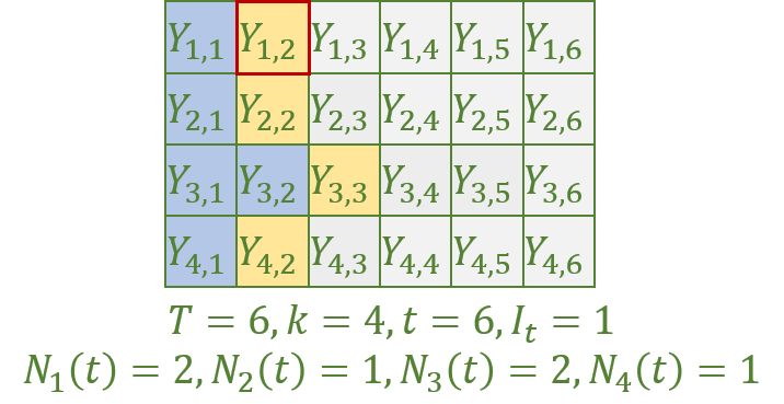
Let $\vec Y_i$ be the random reward vector whose elements are i.i.d. random variables from $D_i$ :

$\vec Y_i = (Y_{i, 1}, Y_{i, 2}, ..., Y_{i, T})$

Denote $Y$ be the matrix of the random variables

$Y = \begin{bmatrix} \vec Y_1 \\ \vec Y_2 \\ ... \\ \vec Y_k \end{bmatrix}$

Each time the player pulls the arm, it observes one random variable from the matrix. Specially, let

$I_t:$ the machine played at the $t$ -th trial,
$N_i(t):$ the number of times the machine $i$ is played up to trial $t$ .

Before trial $t$ , the number of random variables observed in $\vec Y_{I_t}$ is $N_{I_t} (t - 1)$ . At trial $t$ , a new random variable in $\vec Y_{I_t}$ is observed, and $N_{I_t} (t) = N_{I_t} (t - 1) + 1$ . Hence, the newly observed random variable is $Y_{I_t, N_{I_t} (t)}$ . For convenience, we define

$X_{t} \doteq Y_{I_t, N_{I_t} (t)}:$ the rewards obtained at the $t$ -th trial.

When the player chooses a machine $I_t$ on trial $t$ , it is based on the history of his play, which consists of his past decisions, and the corresponding observed rewards:

$H_t: \{ (I_1, X_1), (I_2, X_2), ..., (I_{t -1}, X_{t - 1}) \}$ the history up to trial $t$ .

The strategy the player uses at trial $t$ is considered as a functions from $H_t$ to $[k]$ :

$\phi_t: H_t \rightarrow [k]$ a function that chooses a machine based on the history at trial $t$

We define the policy as the strategies the player uses over all trials:

$\phi = (\phi_1, \phi_2, ..., \phi_T):$ policy, the strategy for the pulling arms by the player

The goal is to find a policy that maximizes the expected rewards, or equivalently, the one that minimizes the expected regret

\small \mathbb{R}(\phi) = T \cdot \mu^* - \mathbb{E}[\sum_{t = 1}^T X_t ]

By definition of $N_i(t)$ 's, we have $\sum_{i = 1}^k N_i(T) = T$ . Then the regret can be written as

\mathbb{R}(\phi) = \mathbb{E}[\sum_{i = 1}^k N_i(T)] \cdot \mu^* - \sum_{i = 1}^k \mathbb{E}[N_i(T) ] \cdot \mu_i = \sum_{i : \Delta_i > 0} \mathbb{E}[N_i(T) ] \cdot \Delta_i

The Upper Confidence Bound (UCB) Algorithm

When making decision at trial $t$ , a good indicator of a machine's performance is its empirical reward:

\hat \mu_{i, N_i(t - 1)} \doteq \sum_{\tau = 1}^{N_i(t - 1) } \frac{1}{ N_i(t - 1) } Y_{i, \tau}

But this might not reflect the true value of its expectation $\mu_i$ because of sampling variation. The UCB algorithm takes the variation into consideration.

Fact. Hoeffding Inequality. Let $Z_1, Z_2, ..., Z_s$ be i.i.d. copies of random variable $Z$ on $[a, b]$ . Then

\Pr[ \frac{1}{s} \sum_{\tau = 1}^s Z_\tau - E[Z] \ge r] \le \exp(- \frac{2 s r^2}{(b - a)^2 } )

where r > 0.

Now, consider a fixed $s$ ( $1 \le s \le T$ ) and a failure probability $\delta > 0$ . Applying Hoeffding inequality with $Z_1 = Y_{i, 1}, Z_2 = Y_{i, 2}, ..., Z_s = Y_{i, s}$ , $a = 0, b = 1$ and $r = \sqrt { \log \frac{1}{\delta} \over 2 s }$ , we get

\small \Pr \left[ \hat \mu_{i, s} - \mu_i \ge \sqrt { \log \frac{1}{\delta} \over 2 s } \right] \le \delta

Similarly, by applying Hoeffding inequality with $Z_1 = -Y_{i, 1}, Z_2 = -Y_{i, 2}, ..., Z_s = -Y_{i, s}$ , $a = -1, b = 0$ and $r = \sqrt { \log \frac{1}{\delta} \over 2 s }$ , we have

\small \Pr \left[ \mu_i - \hat \mu_{i, s} \ge \sqrt { \log \frac{1}{\delta} \over 2 s } \right] \le \delta

Inspired by this, the UCB defines the upper and lower bounds for the expected reward of the $i$ -th machine as follows:

\small UB_i ( t ) \doteq \hat \mu_{i, N_i(t - 1)} + \sqrt { \log t^\alpha \over 2 N_i(t - 1) } \\ LB_i ( t ) \doteq \hat \mu_{i, N_i(t - 1)} - \sqrt { \log t^\alpha \over 2 N_i(t - 1) } \\

where $\alpha > 0$ is a parameter to be set. By convention here that if $N_i(t - 1) = 0$ , $\sqrt { \log t^\alpha \over 2 N_i(t - 1) } = \infty$ .

The UCB algorithms chooses just the machine with highest upper bound. The lower bound is needed for its analysis.

UCB algorithm

For $t \leftarrow 1$ to $T$ do

$\qquad$ Choose $I_t = \arg \max_{i \in [k] } UB_i ( t )$

$\qquad$ Observe a reward $X_t$

Intuitively, there are two cases when $UB_i ( t )$ is high:

The value $\mu_i$ is high;
The $i$ -th machine is under-explored.

Caveat: The reader might start to think that at trial $t$ , it holds that $\Pr[\mu_i \ge UB_i(t) ]$ (or $\Pr[\mu_i \le LB_i(t) ]$ ) is bounded by $\frac{1}{t^\alpha}$ , according to Hoeffding inequality. It is not. Hoeffding inequality requires the number of samples to be a fixed number. On the other hand, $N_i(t - 1)$ is a random variable that depends on the history of the game. We will discuss this later.

The following theorem states that the expected regret of UCB algorithm grows logarithmically with $T$ .

Theorem. If $\alpha > 2$ , the regret of the UCB algorithm is bounded by

\small \mathbb{R}(\phi) \le \log T \cdot ( \sum_{i : \Delta_i > 0 } \frac{2 \alpha }{\Delta_i } ) + \frac{\alpha}{ \alpha - 2 } \sum_{i : \Delta_i > 0 } \Delta_i

Proof:

We will show that for $i : \Delta_i > 0$ ,

\small \mathbb{E} [n_{i, T}] \le \frac{ \alpha \log T }{ \Delta_i^2} + \frac{\alpha}{\alpha - 2}

The key for the proof relies on a sufficient condition that the $i$ -th machine will not be chosen at trial $t$ :

if the following events happen at trial $t$ , machine $i$ will not be chosen:

$A_t: 2 \sqrt { \alpha \log t \over 2 N_i(t - 1) } \le \Delta_i$

$B_t: UB_{ i^* } ( t ) > \mu^*$

$C_t: \mu_i > LB_i ( t )$

This condition essentially prevents $UB_i(t)$ from exceeding $\mu^*$ while assures $UB_{i^*}(t)$ is higher than $\mu^*$ .

\small UB_i ( t ) = LB_i ( t ) + 2 \sqrt { \alpha \log t \over 2 N_i(t - 1) } < \mu_i + \Delta_i = \mu^* < UB_{ i^* } ( t )

Let $\beta = \lceil \frac{2 \alpha \log T}{\Delta_i^2} \rceil$ . Note that $A_t = \{ N_i(t - 1) \ge \frac{2 \alpha \log t}{\Delta_i^2} \} \subset \{ N_i(t - 1) \ge \beta \}$ . Now,

\{I_t = i \} \subset \overline{ A_t \cap B_t \cap C_t } = \bar A_t \cup \bar B_t \cup \bar C_t

and

\begin{array}{ll} \mathbb{E}[n_{i, T}] &= \mathbb{E}[ \sum_{t = 1}^T \mathfrak{1} \{I_t = i\} ] \\ &= \mathbb{E} [ \sum_{t = 1}^T \mathfrak{1} \{I_t = i, \bar A_t \}+ \sum_{t = 1}^T \mathfrak{1} \{I_t = i, A_t \} ] \\ &\le \mathbb{E} [ \sum_{t = 1}^T \mathfrak{1} \{I_t = i, \ N_i(t) < \beta \} ] + \sum_{t = 1}^T \mathbb{E} [\mathfrak{1} \{I_t = i, A_t \} ] \\ &\le \beta + \sum_{t = \beta + 1}^T \Pr[ \{I_t = i\} \cap A_t ] \\ &\le \beta + \sum_{t = \beta + 1}^T ( \Pr[ \bar B_t \cap A_t ] + \Pr[ \bar C_t \cap A_t ] ) \\ &\le \beta + \sum_{t = \beta + 1}^T ( \Pr[ \bar B_t ] + \Pr[ \bar C_t ] ) \\ \end{array}

It is non-trivial to bound $\Pr[\bar B_t]$ . For a fixed $1 \le s \le t - 1$ , define the event

M_s : \frac{1}{s} \sum_{\tau = 1}^s Y_{i^*, \tau} + \sqrt{ \frac{\alpha \log t}{2 s} } \le \mu^*

Since $s$ is fixed, by Hoeffding inequality, $\Pr[M_s] \le \frac{1}{t^\alpha}$ . Then

\small \begin{aligned} \bar B_t = \left\{ \mu_{ {i^*}, N_{i^*} (t - 1)} + \sqrt { \alpha \log t \over 2 N_{i^*} (t - 1) } \le \mu^* \right\} \subset \cup_{s = 1}^{t - 1} M_s \end{aligned}

and

\Pr[ \bar B_t ] \le \Pr[ \cup_{s = 1}^{t - 1} M_s ] \le \sum_{s = 1}^{t - 1} \Pr[M_s] < t^{\alpha - 1}

and

\sum_{t = \beta + 1}^T \Pr[ \bar B_t ] < \sum_{t = \beta + 1}^T t^{\alpha - 1} < \int_{t = 1}^\infty \frac{1}{ x^{\alpha - 1} } dx = \frac{1}{\alpha - 2} x^{-(\alpha - 2)} \mid_{t = 1}^\infty = \frac{1}{\alpha - 2}

Similarly, we have

\sum_{t = \beta + 1}^T \Pr[ \bar C_t ] < \frac{1}{\alpha - 2}

Finally,

\begin{aligned} \small \mathbb{E} [n_{i, T}] &\le \beta + \frac{2}{\alpha - 2} \\ &\le \frac{2 \alpha \log T}{\Delta_i^2} + 1 + \frac{2}{\alpha - 2} \\ &= \frac{2 \alpha \log T}{\Delta_i^2} + \frac{\alpha }{\alpha - 2} \end{aligned}

Remark: Can we bound $\Pr[ \bar B_t ]$ as follows:

\begin{array}{ll} \Pr[\bar B_t] &= \sum_{\tau = 1}^{t - 1} \Pr[UB_{ i^* } ( t ) < \mu^* \mid n_{i^*, t} = \tau] \cdot \Pr[n_{i^*, t} = \tau]\\ &= \sum_{\tau = 1}^{t - 1} \frac{1}{t^\alpha} \cdot \Pr[n_{i^*, t} = \tau] \\ &= \frac{1}{t^\alpha} \end{array}

When we know $n_{i^*, t} = \tau$ for some $\tau$ , the $n_{i^*, t}$ rewards from machine $i^*$ can't be viewed as independent samples. E.g., if $t$ is large, the best machines has much larger expected reward than others, and $n_{i^*, t}$ is very small compared to $t$ . Then it is likely machine $i^*$ generates bad rewards in the history. The reward sequence of $i^*$ can't be viewed as a sequence of independent samples from distribution $D_{i^*}$ .

$\blacksquare$

Reference

[1] D. Katselis, B. Miranda, and H. Hu, “Lecture 8: Multi-Armed Bandits”, ECE586 MDPs and Reinforcement Learning, Spring 2019, University of Illinois at Urbana-Champaign.
[2] S. Bubeck and N. Cesa-Bianchi, “Regret Analysis of Stochastic and Nonstochastic Multi-armed Bandit Problems,” arXiv:1204.5721 [cs, stat], Nov. 2012, Accessed: Oct. 19, 2020.