Laplace Distribution and Mechanism

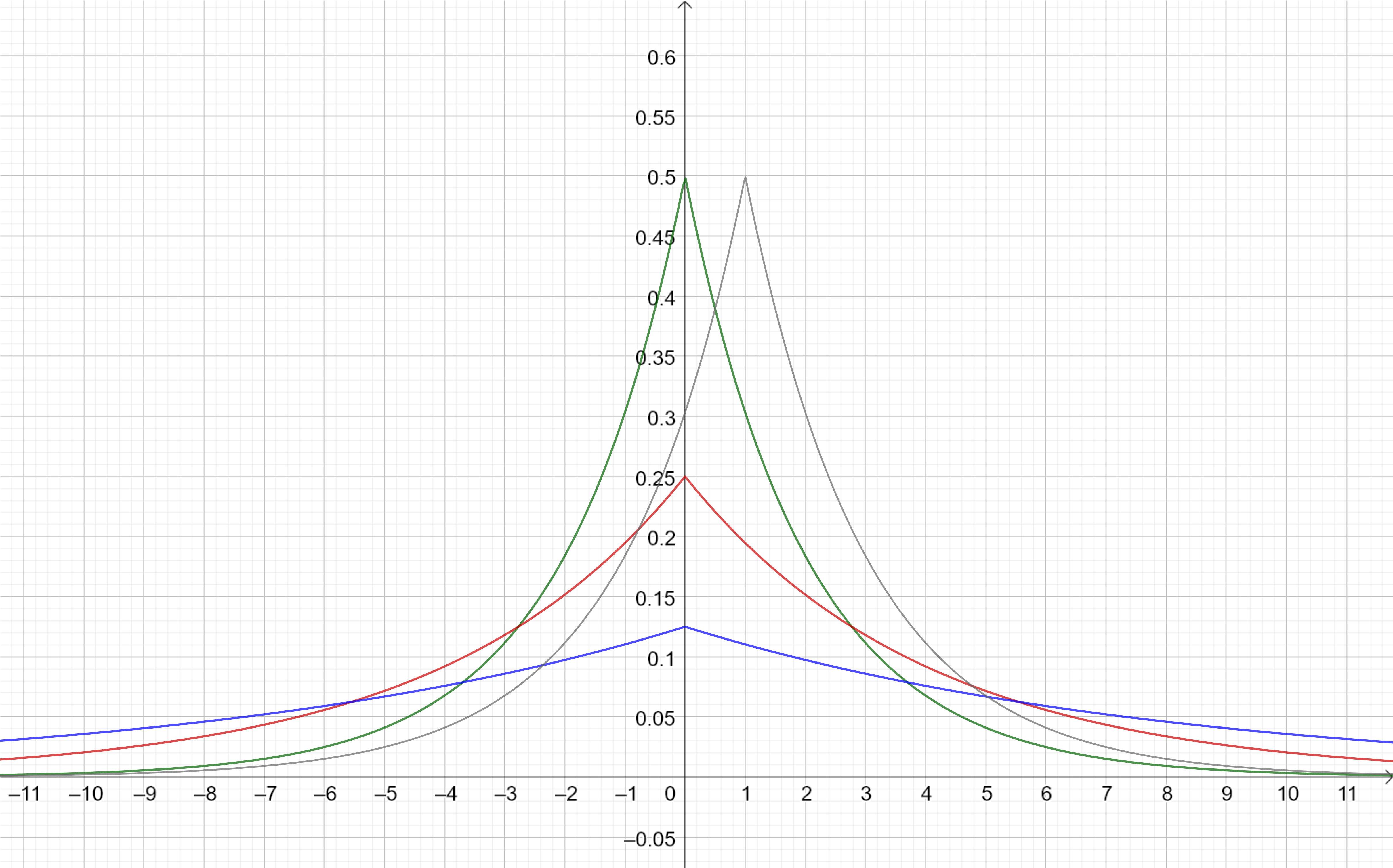
The density function of a Laplace distribution (denoted as Laplace($\mu, b$) ) with location and scale parameters $\mu$ and $b$ is given by

The density function of the distribution is symmetric with respect to $\mu$, where it achieves peak value $\frac{1}{2b}$. We plot below a few Laplace distributions with different parameters of $\mu$ and $b$.

Properties

We list and prove a few properties of the distribution. Let $X$ be a random variable that follows Laplace($\mu, b$).

1. $\mathbb{E}[X] = \mu$.

   Proof.

   $$\small \begin{aligned} \frac{1}{2} \int_{ - \infty }^\infty \frac{1}{2b} x \cdot \exp \left( -\frac{ | x - \mu | }{b} \right) \ dx &= \int_{ - \infty }^\infty \frac{1}{2b} ( x - \mu ) \cdot \exp \left( -\frac{ | x - \mu |}{b} \right) \ dx \\ &+ \int_{ - \infty }^\infty \frac{1}{2b} \mu \cdot \exp \left( -\frac{ | x - \mu |}{b} \right) \ dx \\ &= \int_{\mu }^\infty \frac{\mu}{b} \exp \left( -\frac{x - \mu}{b} \right) \ dx \\ &= \int_{0 }^\infty \frac{ \mu }{b} \exp \left( -\frac{x}{b} \right) \ dx \\ &= \mu. \end{aligned}$$

2. $\forall t \ge 0, \Pr[| X - \mu | \ge b \cdot t] \le \exp(-t)$.
   Proof.

   $$\small \begin{aligned} \Pr[ | X - \mu | \ge t] &= \int_{\mu + b \cdot t }^\infty \frac{1}{b} \exp \left( -\frac{x - \mu}{b} \right) \ dx \\ &= \int_{ b \cdot t }^\infty \exp( -x ) \ dx \\ &= \exp(-t). \end{aligned}$$

   $\square$

3. $\mathbb{Var}[X] = 2b^2$.

   Proof. First, for an integer $n \ge 0$, we define

   $$\Gamma(n) = \int_{0 }^\infty x^n \exp( -x ) \ dx$$

   Therefore, $\Gamma(0) = 1$. Suppose $n \ge 1$, we have

   $$\begin{aligned} \Gamma(n) &= -\int_{0 }^\infty x^n \ d \exp( -x ) \\ &= - x^n \exp(-x) \mid_0^\infty + \int_{0 }^\infty \exp( -x ) \ d x^n \\ &= n\int_{0 }^\infty x^{n - 1} \exp( -x ) \ dx \\ &= n \Gamma(n - 1) \end{aligned}$$

   By induction, we conclude $\Gamma(n) = n!$. Now, consider

   $$\begin{aligned} \frac{1}{2} \int_{\mu }^\infty \frac{1}{b} (x - \mu)^2 \exp \left( -\frac{x - \mu}{b} \right) \ dx &= \frac{1}{2} \int_{0 }^\infty \frac{1}{b} x^2 \exp \left( -\frac{x}{b} \right) \ dx \\ &= \frac{b^2}{2} \int_{0 }^\infty x^2 \exp( -x ) \ dx \\ &= \frac{b^2}{2} \Gamma(2) \\ &= b^2 \end{aligned}$$

   The proof follows from symmetry of Laplace($\mu, b$) at $\mu$.

4. Let $X' \sim Laplace(\mu, b)$ and define another random variable $Y = X' + b$, then the density function of $Y$ shares the same shape with that of $X'$, with its center shifted to the right by distance $b$. To distinguish their density function, denote $p_{X'} (\cdot)$ the one for random variable $X'$ and $p_Y(\cdot)$ the one for $Y$. For any $t \in \mathbb{R}$,

   $$\frac{ p_{X'} (t) }{ p_Y(t) } = \exp( - \frac{ |t - \mu | - | t - ( \mu + b ) | }{ b }) \in [ \exp(-1), \exp(1) \ ]$$

5. If $X, X' \sim Laplace(\mu, \frac{b}{\epsilon} )$ be a pair of independent random variables, and $Y = X' + b$, then

   $$\frac{ p_X(t) }{ p_Y(t) } = \exp \left( - \epsilon \frac{ |t - \mu | - | t - ( \mu + b ) | }{ b } \right) \in [ \exp( -\epsilon ), \exp( \epsilon ) \ ]$$

6. Continued. Let $S$ be any interval in $\mathbb{R}$.

   $$\frac{ \Pr[X \in S] }{ \Pr[Y \in S] } = \frac{ \int_{t \in S} p_X(t) \ dt }{ \int_{t \in S} p_Y(t) \ dt } \in [ \exp( -\epsilon ), \exp( \epsilon ) \ ]$$

7. Continued. Denote $P_X$ and $P_Y$ the probability functions of $X$ and $Y$ respectively. Let $S$ be any Borel set in $\mathbb{R}$.

   $$\frac{ \Pr[X \in S] }{ \Pr[Y \in S] } = \frac{ \int_S 1 \ d P_X }{ \int_S 1 \ d P_Y } \in [ \exp( -\epsilon ), \exp( \epsilon ) \ ]$$

8. Let $X = (X_1, X_2, ..., X_n), X' = (X_1', X_2', ..., X_n')$ be independent random vectors with dimension $n$, where $X_i, X_i' \sim Laplace(0, \Delta / \epsilon )$ (for $1 \le i \le n$) are independent random variables. Let $Y \doteq X' + \mu = (Y_1, Y_2, ..., Y_n)$ be another random vector, such that $Y_i = X_i' + \mu_i$ for $1 \le i \le n$ and $|\mu| = \sum_{i \in [n] } \mu_i \le \Delta$. For any $t \in \mathbb{R}^n$,

   $$\begin{aligned} \frac{ p_X(t) }{ p_Y(t) } &= \frac{ \exp \Big( - \big( \epsilon / \Delta \big) \cdot \sum_{i \in [n] } |t_i| \Big) }{ \exp \Big( - \big( \epsilon / \Delta \big) \cdot \sum_{i \in [n] } |t_i - \mu_i| \Big) } \\ &= \exp \left( - \epsilon \frac{ |t | - | t - \mu| }{ \Delta } \right) \\ &\in \Big[ \exp \Big( - \epsilon \frac{ |\mu| }{ \Delta } \Big) , \exp \Big( \epsilon \frac{ |\mu| }{ \Delta } \Big) \Big] \\ &\subset [ \exp( -\epsilon ), \exp( \epsilon ) \ ] \end{aligned}$$

9. Continued. Let $S \subset \mathbb{R}^n$ be any Borel set. Then

   $$\frac{ \Pr[X \in S] }{ \Pr[Y \in S] } \in [ \exp( -\epsilon ), \exp( \epsilon ) \ ]$$

Laplacian Mechanism

Let $(\mathcal{X}, d)$ be a metric space and $f: \mathcal{X} \rightarrow \mathbb{R}^n$ a function defined on $\mathcal{X}$.

Definition. $x, x' \in \mathcal{X}$ are called neighboring points if $d(x, x') = 1$.

Definition. The sensitivity $\Delta$ of $f$ is defined as

$$\Delta \doteq \max_{x, x' \in \mathcal{X}, d(x, x') = 1} \Vert f(x) - f(x') \Vert_1$$

where $\Vert \cdot \Vert_1$ is the $\ell_1$ distance. In other words, $\Delta$ is the maximum $\ell_1$ distance between the images of two neighboring points.

We now construct a new randomized function, called Laplacian mechanism from $f$, as follows.

Definition. The Laplacian mechanism of $f$ is defined as

$$g(x) = f(x) + Y$$

where $Y = (Y_1, Y_2, ..., Y_n)$ is a random vector with independent random variables $Y_i \sim Laplace(\Delta / \epsilon)$.

$\square$

Theorem. $g$ is $(\epsilon, 0)$-differentially private.

Proof. Let $S \subset \mathbb{R}^n$ be an arbitrary Borel set. We need to prove for any pair of neighboring $x, x' \in \mathcal{X}$,

Denote $p_x$ and $p_{x'}$ the density functions for $g(x)$ and $g(x')$ respectively. It reduces to prove the following property of the density function

But

$\square$