Gaussian Distribution

We show how Gaussian distribution (a.k.a. normal distribution) is constructed and list some of its basic properties.

Suppose we would like to have a distribution in $\mathbb{R}$ , such that

It is centered at the origin.
Its density function decreases exponentially with respect to the square distance to the origin.

Remark: if we replace 2 with "a density function decreases exponentially with the distance to the origin", we obtain Laplace distribution.

The density function $p(x)$ should be inversely and exponentially proportional to $x^2$ :

p(x) \propto \exp(-x^2 )

Denote $M$ the value of

M \doteq \int_{-\infty}^\infty \exp(-x^2) \ dx.

It is easy to check that $M$ is finite. Then the close form of $p(x)$ is

p(x) = \frac{1}{M} \exp(- x^2).

It is easy to verity that $p(x)$ is a valid density function: $\int_{-\infty}^\infty p(x) \ dx = 1$ .

Closed Form

Theorem. $ p(x) = \frac{1}{ \sqrt \pi} \exp( - x^2 ) $ is a density function.

In general, it is not hard to construct a distribution. Let $h(x)$ be any integrable function on a domain $\mathcal{D}$ such that

M = \int_\mathcal{D} h(x) \ dx < \infty

Then we can view $h(x)$ as almost an density function of some distribution. The only obstacle is that $M$ might not be $1$ . However this is easy to fix. We scale the value of $h(x)$ by a constant factor at each point by setting

p(x) = \frac{1}{M} h(x).

In this case, we don't even need to know the exact value of $M$ . We only need to guarantee that

The value of $M$ exists and is finite.

Then we can safely rely on $M$ as a normalized. For example, we know that

\int_0^\infty x^{0.2} e^{-x} \ dx \le \int_0^1 e^{-x} \ dx + \int_1^\infty x e^{-x} \ dx < \infty.

We can construct a density function as discussed above. It turns out that this is a special case of Gamma distribution.

For Gaussian distribution, we are lucky as the closed form of $M$ does exists, due to the following "squaring trick":

\begin{aligned} M^2 &= \Big( \int_{-\infty}^\infty \exp( -x^2 ) \ dx \Big)^2 \\ &= \int_{-\infty}^\infty \exp( -x^2 ) \ dx \ \cdot \int_{-\infty}^\infty \exp( -y^2 ) \ dy \\ &= \int_{-\infty}^\infty \int_{-\infty}^\infty \exp( -(x + y) ^2 ) \ dx dy. \end{aligned}

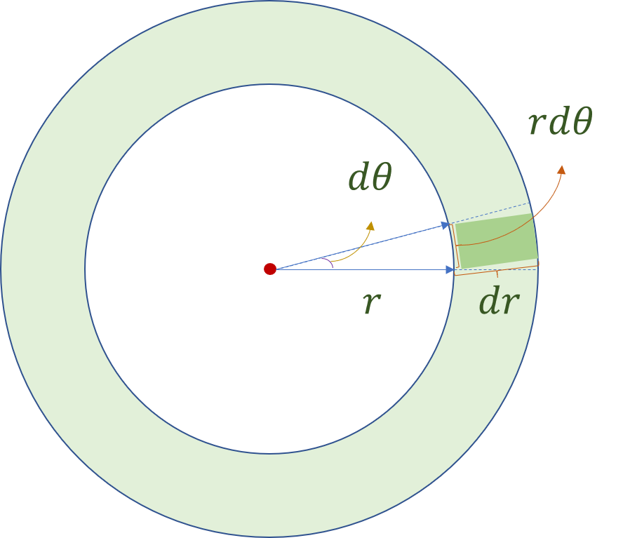
Denote $r \doteq \sqrt{ x^2 + y^2}$ the distance of $(x, y)$ to $(0, 0)$ . We are integrating the function $\exp( - r^2)$ over the plane $\mathbb{R}^2$ . It is natural to switch to polar coordinate system $(r, \theta)$ , where $\theta$ is the angle of a point. Here is an informal but intuitive explanation. As the picture below demonstrates, if $r$ increases by $dr$ and $\theta$ increases by $d\theta$ , the new area spanned by $dr$ and $d \theta$ is roughly $r dr d \theta$ .
We can also calculate this algebraically

\frac{1}{2} [(r + dr)^2 - r^2] d\theta = r dr d \theta + \frac{1}{2} (dr)^2 d \theta \approx r dr d \theta.

Finally,

\begin{aligned} M^2 &= \int_{0}^{ 2 \pi} \int_{0}^\infty \exp( -r^2 ) r d r d \theta \\ &= \int_{0}^{ 2 \pi} \frac{1}{2} \int_{0}^\infty \exp( -r^2 ) d r^2 d \theta \\ &= \int_{0}^{ 2 \pi} \frac{1}{2} d \theta \\ &= \pi. \end{aligned}

Basic Properties

Expectation

As the distribution is symmetric to $0$ , it has expectation 0.

Variance

As its expectation is 0, the variance is given by

\begin{aligned} \int_{-\infty}^\infty \frac{ x^2 }{ \sqrt \pi } \exp( -x^2 ) \ dx &= -\frac{1}{2 \sqrt \pi } \int_{-\infty}^\infty x \ d \exp( -x^2 ) \\ &= \frac{1}{2 \sqrt \pi } \int_{-\infty}^\infty \exp( -x^2 ) d x\\ &= \frac{1}{2 \sqrt \pi } \sqrt \pi \\ &= \frac{1}{2} \end{aligned}

General Gaussian Distribution

We have proved that if $X$ is a random variable with density function $p(x) = \frac{1}{\sqrt \pi} \exp( -x^2)$ , then

\mathbb{Var}[X] = \frac{1}{2}.

Define another random variable $Y \doteq \sqrt{2} X$ , whose variance is

\mathbb{Var}[X] = 2 \mathbb{Var}[X] = 1.

To obtain its density function of $Y$ , we first scale the function $p(x)$ horizontally by a factor of $\sqrt 2$ to get

\frac{1}{ \sqrt{ \pi } } \exp \Big( -\frac{x^2}{2} \Big).

Now the area under the curve $f(x) = \frac{1}{ \sqrt{ \pi } } \exp \big( - x^2 / {2} \big)$ is $\sqrt 2$ . We normalize this area to $1$ and obtain $Y$ 's density function as

p(y) = \frac{1}{ \sqrt{2 \pi } } \exp \Big( -\frac{y^2}{2} \Big)

In what follows, we use $N(0, 1)$ to denote a Gaussian distribution with mean 0 and variance $1$ . We can also scale $X$ by a factor of $\sqrt 2 \sigma$ for any $\sigma > 0$ , to get $Y = \sqrt 2 \sigma X$ . It have variance $\sigma^2$ and density function

p(y) = \frac{1}{ \sqrt{2 \pi \sigma^2} } \exp \Big( - \Big(\frac{y}{ \sqrt{2} \sigma } \Big)^2 \Big) = \frac{1}{ \sqrt{2 \pi \sigma^2 } } \exp \Big( -\frac{y^2}{ 2 \sigma^2 } \Big).

Finally, we can shift the center of $0$ by any real number $\mu \in \mathbb{R}$ to obtain a new density function

p(y) = \frac{1}{ \sqrt{ \pi \cdot 2 \sigma^2 } } \exp\Big( -\frac{ (y - \mu)^2 }{ 2 \sigma^2 } \Big).

The corresponding distribution is denoted as $N(\mu, \sigma^2)$ .

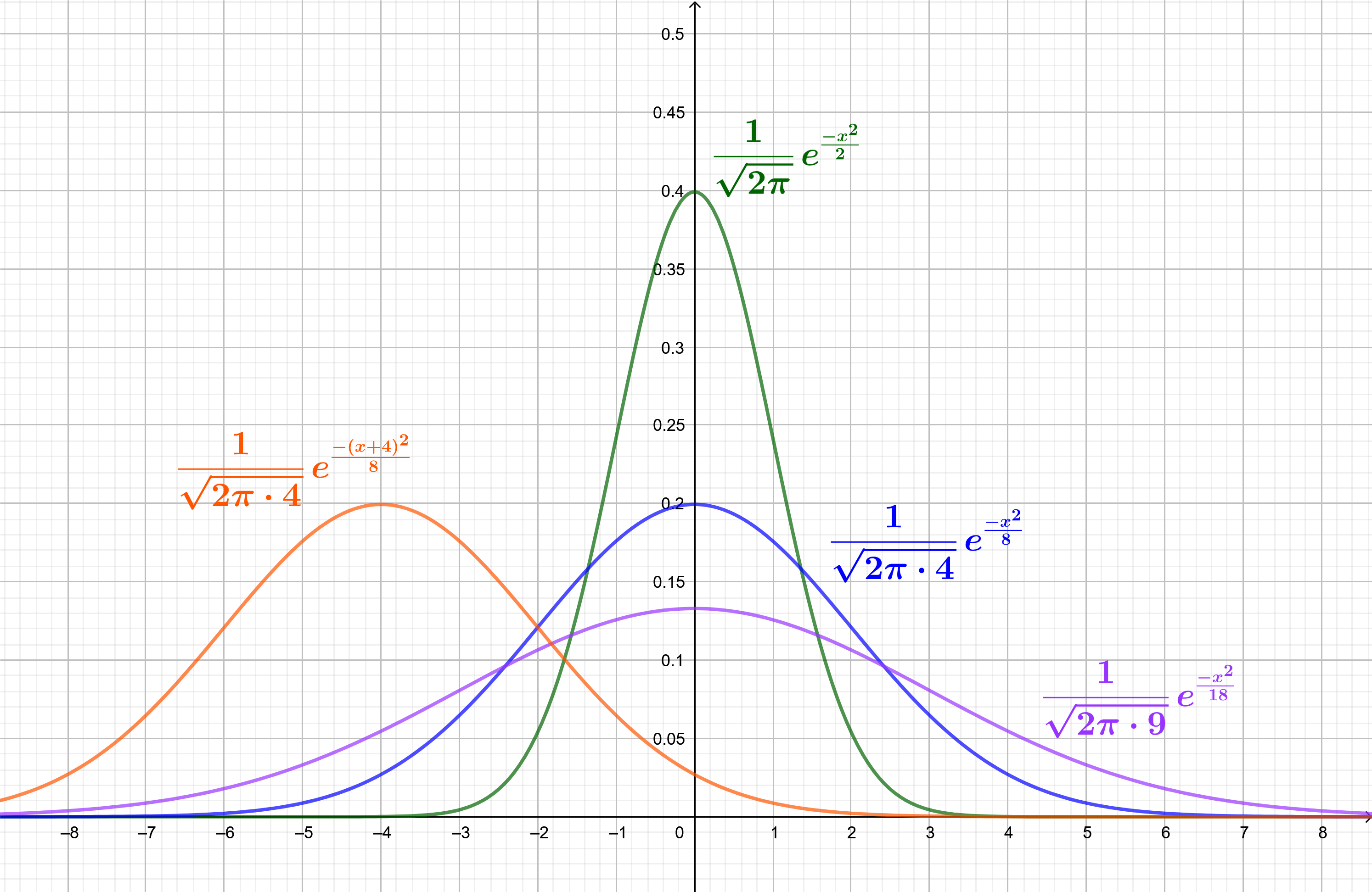
The picture below shows a few Gaussian distributions.

Advanced Properties

Sum of Normal Random Variables

If $X \sim N(\mu_1, \sigma_1^2)$ and $Y \sim N(\mu_2, \sigma_2^2)$ , then for each $a, b \in \mathbb{R}$ ,
$a X + b Y \sim N(a \mu_1 + b \mu_2 , a^2 \sigma_1^2 + b^2 \sigma_2^2).$

Let $X', Y' \sim N(0, 1)$ . Then $X = \mu_1 + \sigma_1 X'$ and $Y = \mu_2 + \sigma_2 Y'$ , and

a X + b Y = a \mu_1 + b \mu_2 + a \sigma_1 X' + b \sigma_2 Y'.

It suffices to prove that if $X', Y' \sim N(0, 1)$ ,

a \sigma_1 X' + b \sigma_2 Y' \sim N(0, a^2 \sigma_1^2 + b^2 \sigma_2^2), \quad \forall a, b \in \mathbb{R}, \forall \sigma_1, \sigma_2 \in \mathbb{R}_{\ge 0}.

Hence, we can assume without lose of generality that $X, Y \sim N(0, 1)$ , and prove that $a X + bY \sim N(0, a^2 + b^2)$ for each $a, b \in \mathbb{R}$ .

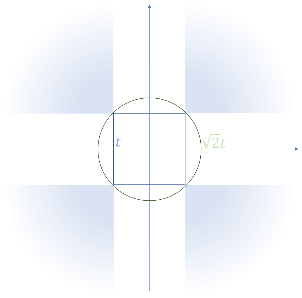
The demonstration here follows from [1]. The key observation is that if $X, Y \sim N(0, 1)$ , the joint distribution of $X$ and $Y$ is rotation invariant with the origin.

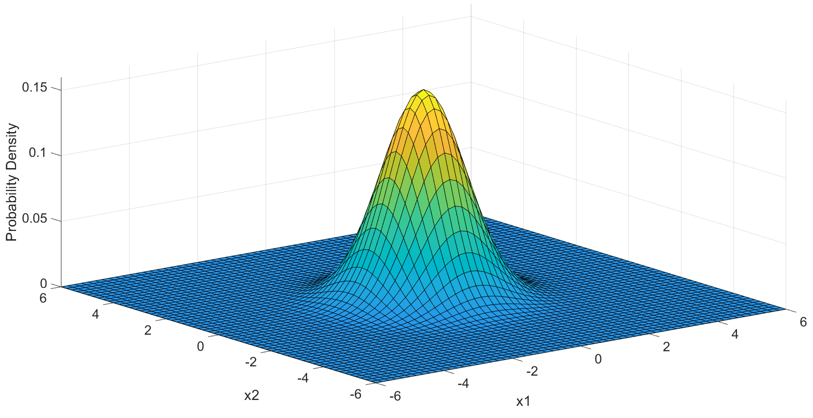
The figure below shows the same distribution. Observe again that the probability mass concentrates at a small region centered at origin.

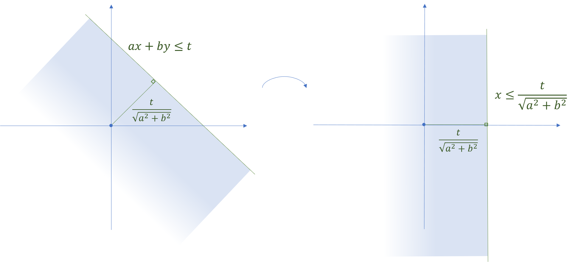
Therefore, for any $t \in \mathbb{R}$ , the set

\{ (x, y) \in \mathbb{R}^2 : ax + by \le t \}

has the same probability measure as the one

\Big\{ (x, y) \in \mathbb{R}^2 : x \le \frac{ t}{ \sqrt{a^2 + b^2} } \Big\}.

Observe that the latter can be obtained by rotating the former with respect to the origin (see the figure below).

Now, the probability of the latter set is given by

\Pr \Big[ X \le \frac{ t}{ \sqrt{a^2 + b^2} } \Big] = \Pr\Big[ \sqrt{a^2 + b^2} X \le t \Big]

It concludes that $X + Y$ has the same distribution as $\sqrt{a^2 + b^2} X \sim N(0, a^2 + b^2)$ .

Concentration Inequalities

Bound 1

If $X \sim N(0, \sigma^2)$ , then $\forall t > 0$ ,
$\Pr[ |X| \ge t] \le \exp \Big( -\frac{t^2}{ 2\sigma^2} \Big)$

Remark: it is possible to get a tighter bound by using more advanced techniques.

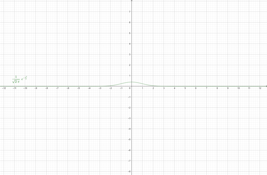
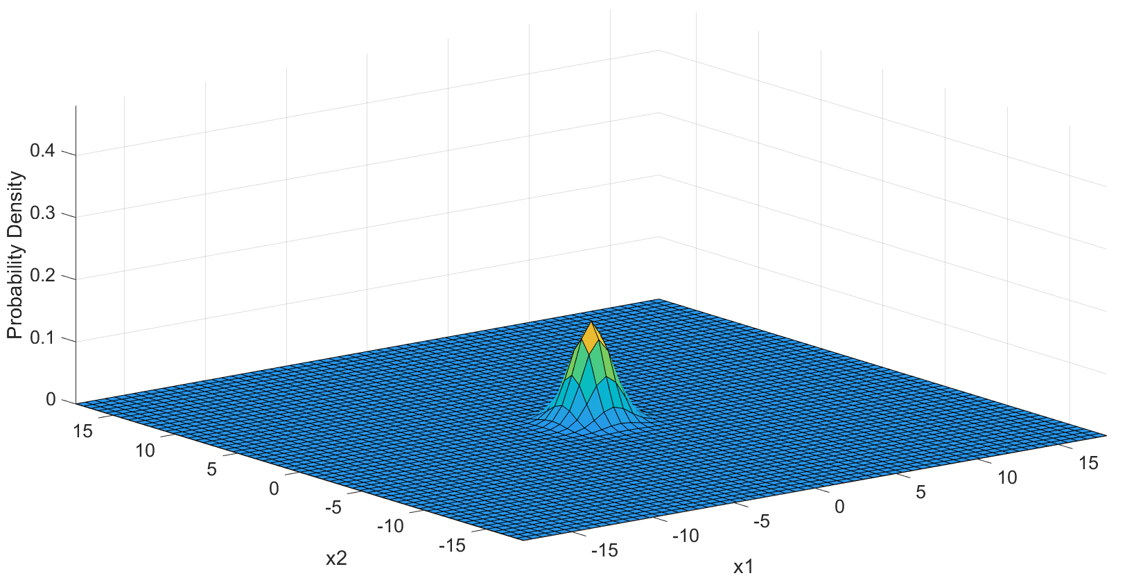
Intuition: in previous figures, it seems Gaussian distributions have a shape bump around its mean. This is kind of mis-leading, because the x-axis and y-axis are scaled. In the figure below, we plot $N(0, 1)$ , with ratio between $x$ and $y$ axes being approximate $1:1$ . We see only a small bump around its mean. Although the distribution span the entire range of $\mathbb{R}$ , the probability mass is centered tightly around the origin.

Proof by Moment Generating Function

We prove a weaker version by a factor of $2$ . For all $\lambda \in \mathbb{R}$ ,

\begin{aligned} \mathbb{E}[ e^{\lambda X} ] &= \frac{1}{\sqrt{2 \pi \sigma} }\int e^{\lambda x} e^{ - \frac{x^2}{2 \sigma^2 } } \ d x \\ &= \frac{ e^{\lambda^2 \sigma^2 / 2} }{\sqrt{2 \pi \sigma} }\int e^{ - \frac{ (x - \lambda \sigma^2)^2}{2 \sigma^2 } } \ d x \\ &= e^{\lambda^2 \sigma^2 / 2}. \end{aligned}

Via Markov's inequality, for all $\lambda \ge 0$ , we have

\begin{aligned} \Pr[ X \ge t] &\le \frac{ \mathbb{E}[ e^{\lambda X} ] }{ e^{\lambda t} } &\le e^{\lambda^2 \sigma^2 / 2 - \lambda t}. \end{aligned}

Setting $\lambda = \frac{t}{\sigma^2}$ , we get

\Pr[ X \ge t ] \le e^{ - \frac{t^2}{2 \sigma^2} }.

It concludes that $\Pr[ |X| \ge t ] \le 2 e^{ - \frac{t^2}{2 \sigma^2} }.$

Proof by Geometry

Let $T = \Pr[ |X| \ge t]$ . Then

T^2 = \int_{ |x| \ge t, |y| \ge t} \frac{1}{ 2 \pi \sigma^2 } \exp \Big( - \frac{ x^2 + y^2}{2 \sigma^2} \Big).

\{ (x, y) \in \mathbb{R}^2: |x| \ge t \wedge |y| \ge t \} \subset \{ (x, y) \in \mathbb{R}^2: x^2 + y^2 \ge 2 t^2 \}

It follows that

\begin{aligned} T^2 &\le \int_{ \sqrt 2 t}^\infty \int_{0}^{2 \pi } \frac{1}{ 2 \pi \sigma^2 } \exp \Big( - \frac{ r^2 }{2 \sigma^2} \Big) r \ d\theta dr\\ &\le \int_{ \sqrt 2 t }^\infty \exp \Big( - \frac{ r^2 }{2 \sigma^2} \Big) \ d \frac{r^2}{ 2\sigma^2} \\ &\le \int_{ \frac{ t^2 }{ \sigma^2 } }^\infty \exp ( - z ) \ d z \\ &= \exp \Big( -\frac{t^2}{ \sigma^2} \Big). \end{aligned}

Therefore,

T \le \exp \Big( - \frac{t^2}{ 2\sigma^2} \Big).

Bound 2

If $X \sim N(0, \sigma^2)$ , then $\forall t > 0$ ,
$\Pr[ X \ge t] \le \frac{ \sigma }{ \sqrt{2 \pi } t } \exp \Big( -\frac{t^2}{ 2\sigma^2} \Big).$
By symmetry we also have
$\Pr[ X \le -t] \le \frac{ \sigma }{ \sqrt{2 \pi } t } \exp \Big( -\frac{t^2}{ 2\sigma^2} \Big).$

Proof.

\begin{aligned} \Pr[X > t] &= \int_{t}^\infty \frac{1}{ \sqrt{2 \pi \sigma^2} } \exp \Big( - \frac{ x^2 }{ 2 \sigma^2 } \Big) \ dx \\ &\le \int_{t}^\infty \frac{1}{ \sqrt{2 \pi \sigma^2} } \frac{x}{t} \exp \Big( - \frac{ x^2 }{ 2 \sigma^2 } \Big) \ dx \\ &\le \frac{ \sigma }{ \sqrt{2 \pi } t } \int_{t}^\infty \exp \Big( - \frac{ x^2 }{ 2 \sigma^2 } \Big) \ d \frac{ x^2 }{ 2 \sigma^2 } \\ &= - \frac{ \sigma }{ \sqrt{2 \pi } t } \exp \Big( - \frac{ x^2 }{ 2 \sigma^2 } \Big) \mid_{t}^\infty \\ &= \frac{ \sigma }{ \sqrt{2 \pi } t } \exp \Big( - \frac{ t^2 }{ 2 \sigma^2 } \Big). \end{aligned}

This bound is more useful only when we know that $t \ge \frac{ \sigma }{ \sqrt{2 \pi } }$ .

Reference

[1] B. Eisenberg and R. Sullivan, “Why Is the Sum of Independent Normal Random Variables Normal?,” Mathematics Magazine, vol. 81, no. 5, pp. 362–366, Dec. 2008