PAC Learning Basic

We discuss a toy model of probably approximately correct (PAC) learning [1]. The setting focuses on a $d$-dimension Boolean hypercube $\{0, 1\}^d$ and a set of functions $\mathcal{H} = \{ h : \{0, 1\}^d \rightarrow \{0, 1 \} \}$. A function $h \in \mathcal{H}$ is called a hypothesis or a concept, which assigns each vertex in the hypercube a label 0 or 1.

The goal of PAC learning is to learn an unknown hypothesis, denoted as $h^* \in \mathcal{H}$, from a dataset, which consists of $n$ points $X_1, X_2, \ldots, X_n \in \{0, 1\}^n$ sampled independently from an unknown distribution $D$ (over the hypercube), as well as their labels $Y_1 = h^*(X_1), Y_2 = h^*(X_2), \ldots, Y_n = h^*(X_n)$.

We can state the algorithm for PAC learning in just one sentence.

Output any hypothesis $h' \in \mathcal{H}$ that is consistent with the sampled dataset, i.e.,

$$h'(X_i) = Y_i, \qquad \forall i \in [n]$$

Such an hypothesis always exists, as $h^*$ satisfies this constraint. We have the classic PAC learning theorem.

Theorem. Let $X \in \{0, 1\}^n$ be a random point sampled from the unknown distribution, then for a given $\delta \in (0, 1)$,

$$\Pr[ h'(X) \neq h^*(X)] \ge \sqrt{ \log |\mathcal{H}| + \log \frac{ 1 }{ \delta } \over 2n}$$

with probability at most $\delta$.

The PAC learning theorem states that the probability that $h'$ mislabels a point is bounded by $\sqrt{ \log |\mathcal{H}| + \log ( 1 / \delta ) \over 2n}$.

Proof. Consider some fixed $h \in \mathcal{H}$. For convenience, we rewrite

Denote $Z_i$ the indicator variable of whether $h$ mislabels $X_i$, i.e.,

By definition, $\mathbb{E}[Z_i]$ is an unbiased estimator of $\mu_h$. Further, denote $\hat \mu_h$ the empirical mean of $Z_i$'s

Note that for the outputted $h'$, $\hat \mu_{h'} = 0$.

By Hoeffding inequality, for any $\delta' > 0$,

By union bound, the probability that

is bounded by $| \mathcal{H} | \delta'$. By setting $\delta' = \frac{\delta}{ | \mathcal{H} | }$, it is guaranteed that with probability at most $\delta$,

$\blacksquare$

The previous theorem can be improved with the $\sqrt{ \cdot }$ removed. The key here is that the selected $h'$ is error-free on the samples.

Theorem. Let $X \in \{0, 1\}^n$ be a random point sampled from the unknown distribution, then for a given $\delta \in (0, 1)$,

$$\Pr[ h'(X) \neq h^*(X)] \ge { \log |\mathcal{H}| + \log \frac{ 1 }{ \delta } \over n}$$

with probability at most $\delta$.

Proof. Consider some fixed $h \in \mathcal{H}$. For convenience, we rewrite

We will prove that if $\mu_h \ge { \log |\mathcal{H}| + \log \frac{ 1 }{ \delta } \over n}$, then $h$'s probability of being selected is very low.

Denote $Z_i$ the indicator variable of whether $h$ mislabels $X_i$, i.e.,

By definition, $\Pr[Z_i = 1] = \mu_h$. Therefore,

Taking union bound over all possible $h$ gives the desired result.

$\blacksquare$

Caveat. In both theorem, we see a $\log \mathcal{H}$ term in the failure probability, which is due to the use of union bound and can be roughly considered as the complexity of the hypothesis family. It is tempting to think that this could be avoid as follows.

For the outputted $h'$, $Z_1, \ldots, Z_n$ are i.i.d samples. Therefore, the probability of all of them being $0$ is give by

$$(1 - \mu_{h'} )^n \le \exp( - \mu_{h'} n).$$

Bounding this probability by $\delta$ gives $\mu_{h'} \le \frac{ \log ( 1 / \delta ) } {n}$.

The argument is wrong. For the outputted $h'$, the $Z_1, \ldots, Z_n$ are not i.i.d samples, as $h'$ is selected according to $Z_1, \ldots, Z_n$ and depends on them.

To make it more concrete, suppose that there is an $h$, such that $\mu_h = \frac{ \log ( 1 / \delta ) } {n}$. Consider the following experiment

1. Sample $n$ points independently the distribution $D$.
2. Pick an $h'$ that makes no prediction error on the samples.

If we repeat the experiment $N$ times for some positive integer $N$, then the fixed $h$ makes no mistake in roughly $(1 - \delta) N$ of the experiments and constitutes an candidate of $h'$. However, on the other roughly $\delta N$ experiments, where $h$ makes prediction error, it is no longer considered as the candidate of $h'$. The selection procedure of $h'$ ignores bad event of $h$ automatically.

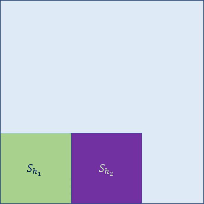
We could also investigate the following example. Let $h^* = h_0$. There are also other two hypothesis $h_1$ and $h_2$. Let $S$ be the sample space. It holds that

Moreover, $\Pr[S_{h_1}] = \Pr[S_{h_2} ] = \delta$. How, if we get a sample in $S_{h_1}$, then we can output $h'$ as $h_0$ or $h_1$, since both of them make no error when $x \in S_{h_1}$. Similarly, if $x \in S_{h_2}$, we can output either $h_0$ or $h_2$. We call $S_{h_1}$ and $S_{h_2}$ the bad areas. When $x$ is in the bad area of any hypothesis, we can't distinguish this hypothesis from the true hypothesis. That is why we need to use union bound to bound the total probabilities of these bad areas.

Reference

[1] Leslie G. Valiant. A theory of the learnable. Communications of the ACM, 27(11):1134-1142, 1984. 6