Complex Numbers

I feel uncomfortable with complex numbers for a long time, partially because of the way they are introduced in the textbooks. They are considered necessary for solving equations such as

Somehow magically, a symbol $i$ is introduced, and its square $i^2$ is manually defined as $-1$. Following this, typically a set of operations defined on complex numbers as well as their properties are listed by the textbooks, leaving the question of why we can have such "magical symbol" unsolved.

In this blog, I am trying to introduce complex numbers in a more natural manner, by studying rotations, dilations and additions of points in $\mathbb{R}^2$. I will show that these operations satisfy some properties, such that we can manipulate points in $\mathbb{R}^2$ in a similar way as real numbers (by addition and multiplication).

We first reflect on the real numbers $\mathbb{R}$. They are concrete, since they can be represented by points on the real axis. We can perform addition ($+$) and multiplication ($\cdot$) on them, that satisfy the following properties (referred to as field axioms). Let $a, b, c \in \mathbb{R}$,

1. Associativity of addition: $a + (b + c) = (a + b) + c$.
2. Commutativity of addition: $a + b = b + a$.
3. Additive identity: there exists a 'zero' element $0$ such that $a + 0 = a$.
4. Additive inverse: there is an element, denoted as $-a$, such that $a + (-a) = 0$.
5. Associativity of multiplication: $a \cdot (b \cdot c) = (a \cdot b) \cdot c$.
6. Commutativity of addition: $a \cdot b = b \cdot a$.
7. Multiplicative identity: there exists a 'one' element $1$ such that $a \cdot 1 = a$.
8. Multiplicative inverse: there exists a element $a^{-1}$ for $a \neq 0$ such that $a \cdot a^{-1} = 1$.
9. Distributivity: $a \cdot (b + c) = a \cdot b + a \cdot c$.

Any set with two operations that satisfy similar properties as above is called a field. In the remainder of the blog, we show how to construct a field from $\mathbb{R}^2$.

We can view $\mathbb{R}^2$ as the set of vectors that originates from the origin. Hence, each element in $\mathbb{R}^2$ is considered as both a point and a vector. We will define addition and multiplication for $\mathbb{R}^2$. For the moment, we will use $\oplus$ and $\odot$ to denote addition and multiplications in $\mathbb{R}^2$, to distinguish the operations $+$ and $\cdot$ for $\mathbb{R}$. Lastly, we show that the set system $(\mathbb{R}^2, \oplus, \odot)$ constitutes a field.

In the remainder of the blog, when we refer to a vector, we refer to the one that originate from the origin.

Addition $\oplus$

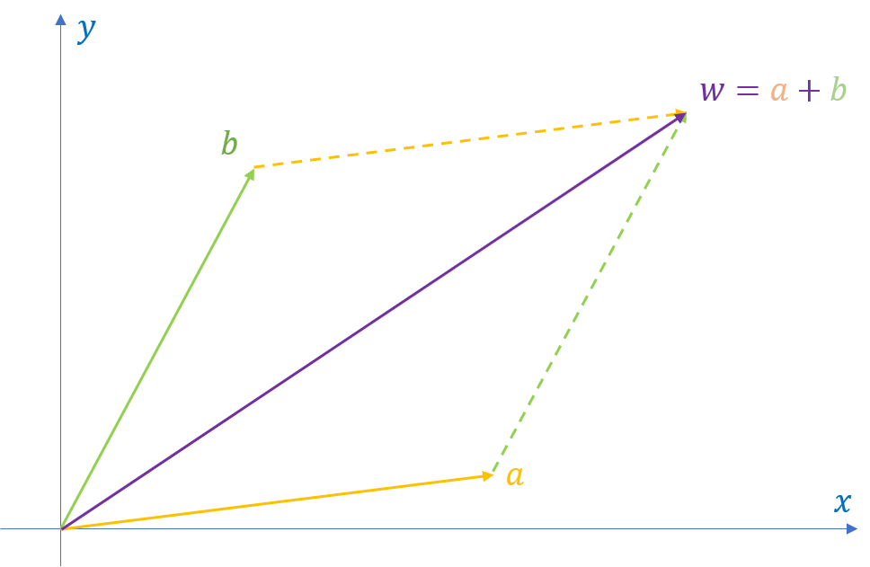
Addition in $\mathbb{R}^2$ is defined the same way as vector addition. When points are specified by Cartesian coordinates, it is easy to get a closed form expression of addition. Let $a = (a_1, a_2), b = (b_1, b_2) \in \mathbb{R}^2$, then

Multiplication $\odot$

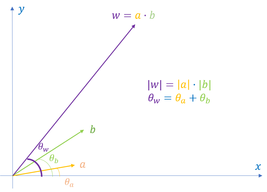
When multiplying two vectors, their lengths multiply and their angles add. It is an operation that involves both dilation and rotation.

We investigate multiplication in the polar coordinates. For $a \in \mathbb{R}^2$, let $|a| \in \mathbb{R}$ be its length and $\theta_a$ be its angle with respect to the $x$-axis. We can write $a$ as:

For $a, b \in \mathbb{R}^2$,

The result is a vector (from the origin) with length $|a| \cdot |b|$ and angle $\theta_a + \theta_b$.

Remark: we have use different coordinate systems to get closed form formulas for addition and multiplication separately. This is immaterial. We need only to make sure both addition and multiplication are functions in $\mathbb{R}^2 \times \mathbb{R}^2 \rightarrow \mathbb{R}^2$. Writing the closed form of a function in a coordinate system is just a specific way to describe it. For a specific function $f$ in $\mathbb{R}^2 \times \mathbb{R}^2 \rightarrow \mathbb{R}^2$, it maps each pair of $a, b \in \mathbb{R}^2 \times \mathbb{R}^2$ to a unique point $f(a, b) \in \mathbb{R}^2$, whether this function is described in Cartesian or polar coordinates. If we want, we can even describe it by language. For example, the sentence "$f$ takes every pair of $\forall a, b \in \mathbb{R}^2$ to the origin." defines a constant function.

Field Verification

We need to verify that the set system $(\mathbb{R}^2, \oplus, \odot)$ is a field.

1. Associativity of addition: $a \oplus (b \oplus c) = (a \oplus b) \oplus c$

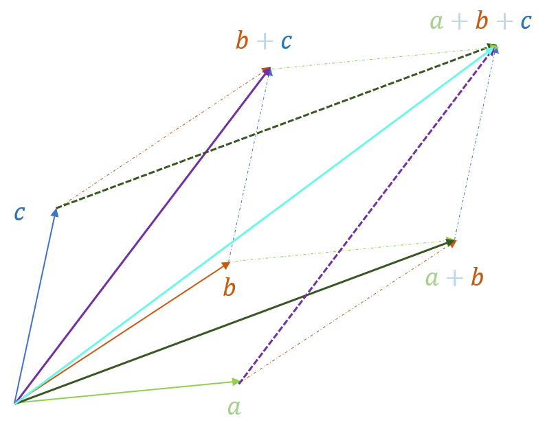
The figure below shows that addition is associative.

Associativity is also easy to verify in Cartesian coordinates. Let $a = (a_1, a_2), b = (b_1, b_2), c = (c_1, c_2)$, we get

$\square$

2. Commutativity of addition: $a \oplus b = b \oplus a$

This is verified when we define addition or we can check it easily in Cartesian coordinate system.

$\square$

3. Additive identity: $\exists$ $\vec 0$, s.t. $a \oplus \vec 0 = a$

$(0, 0) \in \mathbb{R}^2$ serves as the zero element.

$\square$

4. Additive inverse: $\exists (-a) \in \mathbb{R}^2$, s.t. $a \oplus (-a) = \vec 0$

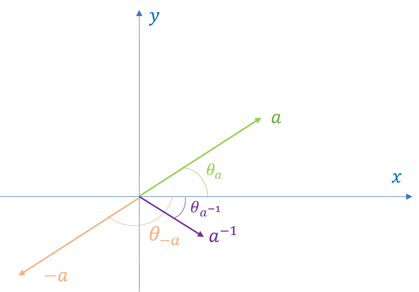
Let $(-a)$ be the vector that is symmetric to $a$ with respect to the origin. Then $a \oplus (-a) = 0$. Indeed, if $a = (a_1, a_2)$,

$\square$

5. Associativity of multiplication: $a \odot (b \odot c) = (a \odot b) \odot c$

It is more convenient to check the properties involved multiplication via polar coordinates.

$\square$

6. Commutativity of addition: $a \odot b = b \odot a$

Similarly,

$\square$

7. Multiplicative identity: $\exists \vec 1$ s.t. $a \odot \vec 1 = a$

$(1, 0) = |1|\angle 0$ is the 'one' vector.

$\square$

8. Multiplicative inverse: If $a \neq \vec 0$, $\exists a^{-1}$, s.t. $a \odot a^{-1} = \vec 1$

The multiplicative inverse is given by

$\square$

9. Distributivity: $a \odot (b \oplus c) = a \odot b \oplus a \odot c$

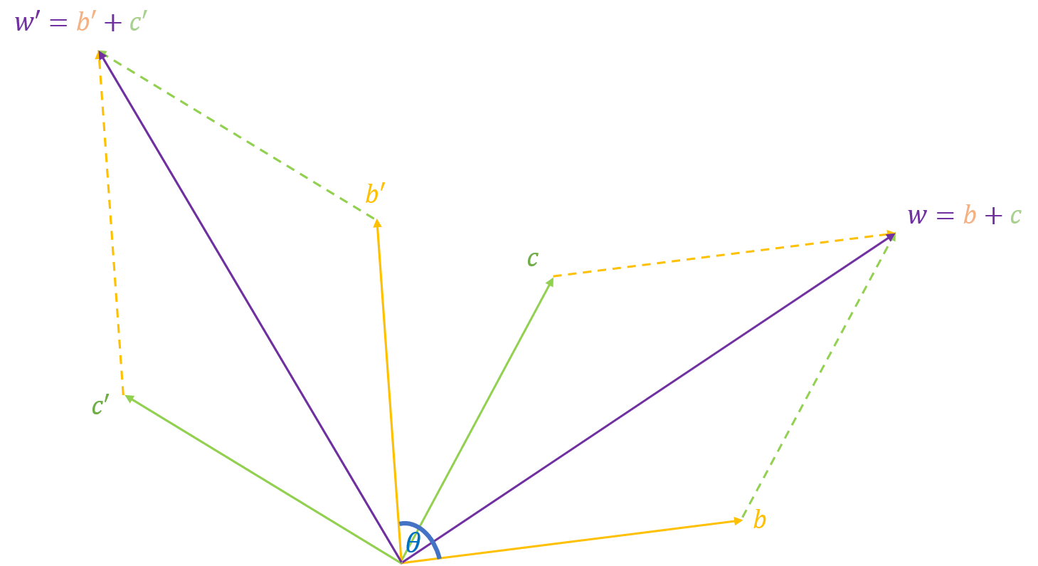
Distributivity involves both addition and multiplication. We prove it geometrically.

Let $w = b \oplus c$.

First suppose $|a| = 1$. In such case, $a = |1| \angle \theta_a$ and

Multiplying $w$ by $a$ is equivalent to rotating it by an angle of $\theta_a$. Let $w', b', c'$ be the vectors obtained by rotating $b, c, w$ by angle $\theta_a$. Then

The figure belows show that

In case $|a| > 1$, $|w'|$, $|b'|$ and $|c'|$ are magnified by a factor of $|a|$ and the same conclusion apply.

$\square$

Conclusion

We have shown that $(\mathbb{R}^2, \oplus, \odot)$ is indeed a field. For convenience, we use $\mathbb{C}$ to denote this set system. If we define

Hence, $\vec j = \vec 1$ and

1. $\vec j \odot \vec j = \vec 1$,
2. $\vec i \odot \vec j = \vec j \odot \vec i = \vec i$,
3. $\vec i \odot \vec i = |1| \angle ( \pi / 2 + \pi / 2) = (-1, 0) = -\vec j$.

For $a = (a_1, a_2), b = (b_1, b_2) \in \mathbb{R}^2$, we can write

and

To derive a formula for multiplication, we use the distributivity property of the two operations

We are almost done. We now further simplify the notations. As $\vec j$ plays the role of $\vec 1$, we can omit it. For $a = (a_1, a_2)$, we use only $\vec i$ to distinguish its $y$-coordinate from the $x$-coordinate:

Addition and multiplication can be performed correctly in this representation:

1. $a \oplus b = a_1 \oplus a_2 \vec i \oplus b_1 \oplus b_2 \vec i = (a_1 + b_1) \oplus (a_2 + b_2) \vec i$.
2. $$\begin{aligned} a \odot b &= a \odot ( b_1 \oplus b_2 \vec i ) \\ &= a \odot b_1 \oplus a \odot (b_2 \vec i) \\ &= (a_1 \oplus a_2 \vec i) \odot b_1 \oplus (a_1 \oplus a_2 \vec i) \odot (b_2 \vec i) \\ &= (a_1 \cdot b_1) \oplus (a_2 \cdot b_1) \vec i \oplus (a_1 \cdot b_2) \vec i \oplus (a_2 \cdot b_2) (\vec i \odot \vec i) \\ &= (a_1 \cdot b_1) \oplus (a_2 \cdot b_1) \vec i \oplus (a_1 \cdot b_2) \vec i \oplus (- a_2 \cdot b_2) \\ &= (a_1 \cdot b_1 - a_2 \cdot b_2) \oplus (a_2 \cdot b_1 + a_1 \cdot b_2) \vec i. \\ \end{aligned}$$

Finally, observe that if we restrict $\oplus$ and $\odot$ to the points on the $x$-axis, they perform similarly as $+$ and $\cdot$ do for $\mathbb{R}$. If we do not distinguish a number $(a_1, 0) \in \mathbb{R}^2$ and $a_1 \in \mathbb{R}$, replace $\oplus$ and $\odot$ with $+$ and $\cdot$, we get exactly the same formula for standard complex number addition and multiplication: $\forall a, b \in \mathbb{R}^2$,

1. $a + b = (a_1 + b_1) + (a_2 + b_2) \vec i$,
2. $a \cdot b = (a_1 + a_2 \vec i) \cdot (b_1 + b_2 \vec i) = (a_1 \cdot b_1 - a_2 \cdot b_2) + (a_1 \cdot b_2 + a_2 \cdot b_1) \vec i$.