In the discrete Fourier transform, we want to project a vector v ∈ C n v \in \mathbb{C}^n v ∈ C n
e 0 = 1 n ( e 0 ⋅ 2 ⋅ 0 ⋅ π i n , e 1 2 ⋅ 0 ⋅ π i n , . . . , e ( n − 1 ) ⋅ 2 ⋅ 0 ⋅ π i n ) , . . . e k − 1 = 1 n ( e 0 ⋅ 2 ⋅ ( k − 1 ) ⋅ π i n , e 1 2 ⋅ ( k − 1 ) ⋅ π i n , . . . , e ( n − 1 ) ⋅ 2 ⋅ ( k − 1 ) ⋅ π i n ) , . . . e n − 1 = 1 n ( e 0 ⋅ 2 ⋅ ( n − 1 ) ⋅ π i n , e 1 2 ⋅ ( n − 1 ) ⋅ π i n , . . . , e ( n − 1 ) ⋅ 2 ⋅ ( n − 1 ) ⋅ π i n ) .
\begin{aligned}
&e_0 = \frac{1}{\sqrt n} \left( e^{ 0 \cdot \frac{2 \cdot 0 \cdot \pi i}{ n} }, e^{ 1 \frac{2 \cdot 0 \cdot \pi i}{ n} }, ..., e^{ (n - 1) \cdot \frac{2 \cdot 0 \cdot \pi i}{ n} } \right), \\
&... \\
&e_{k - 1} = \frac{1}{\sqrt n} \left( e^{ 0 \cdot \frac{2 \cdot (k - 1) \cdot \pi i}{ n} }, e^{ 1 \frac{2 \cdot (k - 1) \cdot \pi i}{ n} }, ..., e^{ (n - 1) \cdot \frac{2 \cdot (k - 1) \cdot \pi i}{ n} } \right), \\
&... \\
&e_{n - 1} = \frac{1}{\sqrt n} \left( e^{ 0 \cdot \frac{2 \cdot (n - 1) \cdot \pi i}{ n} }, e^{ 1 \frac{2 \cdot (n - 1) \cdot \pi i}{ n} }, ..., e^{ (n - 1) \cdot \frac{2 \cdot (n - 1) \cdot \pi i}{ n} } \right).
\end{aligned}
e 0 = n 1 ( e 0 ⋅ n 2 ⋅ 0 ⋅ π i , e 1 n 2 ⋅ 0 ⋅ π i , ... , e ( n − 1 ) ⋅ n 2 ⋅ 0 ⋅ π i ) , ... e k − 1 = n 1 ( e 0 ⋅ n 2 ⋅ ( k − 1 ) ⋅ π i , e 1 n 2 ⋅ ( k − 1 ) ⋅ π i , ... , e ( n − 1 ) ⋅ n 2 ⋅ ( k − 1 ) ⋅ π i ) , ... e n − 1 = n 1 ( e 0 ⋅ n 2 ⋅ ( n − 1 ) ⋅ π i , e 1 n 2 ⋅ ( n − 1 ) ⋅ π i , ... , e ( n − 1 ) ⋅ n 2 ⋅ ( n − 1 ) ⋅ π i ) . We use S \mathcal{S} S e 0 , e 1 , . . . , e n − 1 e_0, e_1, ..., e_{n - 1} e 0 , e 1 , ... , e n − 1
Orthonormal Bases
It is easy to see that e k e_k e k ∀ k ∈ Z n \forall k \in \mathbb{Z}_n ∀ k ∈ Z n k , ℓ ∈ Z n , k ≠ ℓ k, \ell \in \mathbb{Z}_n, k \neq \ell k , ℓ ∈ Z n , k = ℓ
< e k , e ℓ > H = ∑ j ∈ Z n e j ⋅ 2 ( ℓ − k ) π i n = 1 − e n ⋅ 2 ( ℓ − k ) π i n 1 − e 2 ( ℓ − k ) π i n = 0.
\left< e_k, e_\ell \right>_H = \sum_{j \in \mathbb{Z}_n } e^{ j \cdot \frac{ 2 (\ell - k) \pi i }{ n } } = \frac{ 1 - e^{ n \cdot \frac{ 2 (\ell - k) \pi i }{ n } } }{ 1 - e^{ \frac{ 2 (\ell - k) \pi i }{ n } } } = 0.
⟨ e k , e ℓ ⟩ H = j ∈ Z n ∑ e j ⋅ n 2 ( ℓ − k ) π i = 1 − e n 2 ( ℓ − k ) π i 1 − e n ⋅ n 2 ( ℓ − k ) π i = 0. Projection
The projection of v v v v v v
P ( v ) ≐ ∑ k ∈ Z n a k e k ,
P(v) \doteq \sum_{k \in \mathbb{Z}_n} a_k e_k,
P ( v ) ≐ k ∈ Z n ∑ a k e k , where a k = < e k , v > H ≐ e ˉ k ⋅ v a_k = \left< e_k, v\right>_H \doteq \bar e_k \cdot v a k = ⟨ e k , v ⟩ H ≐ e ˉ k ⋅ v
Lemma. For any vector u u u S \mathcal{S} S
< u , v > H = < u , P ( v ) > H .
\left< u, v \right>_H = \left< u, P(v) \right>_H.
⟨ u , v ⟩ H = ⟨ u , P ( v ) ⟩ H . Or, equivalently,
< u , v − P ( v ) > H = < v − P ( v ) , u > H = 0.
\left< u , v - P(v) \right>_H = \left< v - P(v), u \right>_H = 0.
⟨ u , v − P ( v ) ⟩ H = ⟨ v − P ( v ) , u ⟩ H = 0.
Proof. Let u = ∑ k ∈ Z n c k e k : c k ∈ C , ∀ k ∈ Z n u = \sum_{k \in \mathbb{Z}_n} c_k e_k : c_k \in \mathbb{C}, \forall k \in \mathbb{Z}_n u = ∑ k ∈ Z n c k e k : c k ∈ C , ∀ k ∈ Z n S \mathcal{S} S e 0 , e 1 , . . . , e n − 1 e_0, e_1, ..., e_{n - 1} e 0 , e 1 , ... , e n − 1
< u , v > H = ∑ k ∈ Z n c ˉ k ⋅ a k = < u , P ( v ) > H .
\left< u, v \right>_H = \sum_{k \in \mathbb{Z}_n} \bar c_k \cdot a_k =\left< u, P(v) \right>_H.
⟨ u , v ⟩ H = k ∈ Z n ∑ c ˉ k ⋅ a k = ⟨ u , P ( v ) ⟩ H . □ \square □
Next, we verify that P ( v ) P(v) P ( v ) v v v
Theorem.
P ( v ) = arg min w ∈ S ∣ ∣ u − w ∣ ∣ 2 .
P(v) = \argmin_{w \in \mathcal{S} } ||u - w||^2.
P ( v ) = w ∈ S arg min ∣∣ u − w ∣ ∣ 2 .
Proof. Let w = ∑ k ∈ Z n d k e k : d k ∈ C , ∀ k ∈ Z n w = \sum_{k \in \mathbb{Z}_n} d_k e_k : d_k \in \mathbb{C}, \forall k \in \mathbb{Z}_n w = ∑ k ∈ Z n d k e k : d k ∈ C , ∀ k ∈ Z n u = P ( v ) − w u = P(v) - w u = P ( v ) − w u ∈ S u \in \mathcal{S} u ∈ S
∣ ∣ v − w ∣ ∣ 2 = ∣ ∣ v − P ( v ) + P ( v ) − w ∣ ∣ 2 = ∣ ∣ v − P ( v ) ∣ ∣ 2 + ∣ ∣ P ( v ) − w ∣ ∣ 2 + < v − P ( v ) , u > H + < u , v − P ( v ) > H = ∣ ∣ v − P ( v ) ∣ ∣ 2 + ∣ ∣ P ( v ) − w ∣ ∣ 2
\begin{aligned}
|| v - w ||^2
&= || v - P(v) + P(v) - w ||^2 \\
&= || v - P(v) ||^2 + ||P(v) - w||^2 + \left< v - P(v), u \right>_H + \left< u, v - P(v) \right>_H \\
&= || v - P(v) ||^2 + ||P(v) - w||^2
\end{aligned}
∣∣ v − w ∣ ∣ 2 = ∣∣ v − P ( v ) + P ( v ) − w ∣ ∣ 2 = ∣∣ v − P ( v ) ∣ ∣ 2 + ∣∣ P ( v ) − w ∣ ∣ 2 + ⟨ v − P ( v ) , u ⟩ H + ⟨ u , v − P ( v ) ⟩ H = ∣∣ v − P ( v ) ∣ ∣ 2 + ∣∣ P ( v ) − w ∣ ∣ 2 Hence, ∣ ∣ v − w ∣ ∣ 2 || v - w ||^2 ∣∣ v − w ∣ ∣ 2 w = P ( v ) w = P(v) w = P ( v )
□ \square □
The coefficients of a 0 , a 1 , . . . , a n − 1 a_0, a_1, ..., a_{n - 1} a 0 , a 1 , ... , a n − 1
[ a 0 a 1 . . . a n − 1 ] = [ − e ˉ 0 − . . . − e ˉ k − . . . − e ˉ n − 1 − ] v = 1 n [ e − 0 ⋅ 2 ⋅ 0 ⋅ π i n , e − 1 2 ⋅ 0 ⋅ π i n , . . . , e − ( n − 1 ) ⋅ 2 ⋅ 0 ⋅ π i n . . . e − 0 ⋅ 2 ⋅ ( k − 1 ) ⋅ π i n , e − 1 2 ⋅ ( k − 1 ) ⋅ π i n , . . . , e − ( n − 1 ) ⋅ 2 ⋅ ( k − 1 ) ⋅ π i n . . . e − 0 ⋅ 2 ⋅ ( n − 1 ) ⋅ π i n , e − 1 2 ⋅ ( n − 1 ) ⋅ π i n , . . . , e − ( n − 1 ) ⋅ 2 ⋅ ( n − 1 ) ⋅ π i n ] v .
\begin{bmatrix}
a_0 \\
a_1 \\
... \\
a_{n - 1}
\end{bmatrix}
=
\begin{bmatrix}
- \bar e_0 - \\
...\\
- \bar e_k - \\
... \\
- \bar e_{n - 1} - \\
\end{bmatrix} v
=
\frac{1}{ \sqrt n }
\begin{bmatrix}
e^{ -0 \cdot \frac{2 \cdot 0 \cdot \pi i}{ n} }, e^{ -1 \frac{2 \cdot 0 \cdot \pi i}{ n} }, ..., e^{ -(n - 1) \cdot \frac{2 \cdot 0 \cdot \pi i}{ n} } \\
...\\
e^{ -0 \cdot \frac{2 \cdot (k - 1) \cdot \pi i}{ n} }, e^{ -1 \frac{2 \cdot (k - 1) \cdot \pi i}{ n} }, ..., e^{ -(n - 1) \cdot \frac{2 \cdot (k - 1) \cdot \pi i}{ n} } \\
... \\
e^{ -0 \cdot \frac{2 \cdot (n - 1) \cdot \pi i}{ n} }, e^{ -1 \frac{2 \cdot (n - 1) \cdot \pi i}{ n} }, ..., e^{ -(n - 1) \cdot \frac{2 \cdot (n - 1) \cdot \pi i}{ n} } \\
\end{bmatrix} v.
a 0 a 1 ... a n − 1 = − e ˉ 0 − ... − e ˉ k − ... − e ˉ n − 1 − v = n 1 e − 0 ⋅ n 2 ⋅ 0 ⋅ π i , e − 1 n 2 ⋅ 0 ⋅ π i , ... , e − ( n − 1 ) ⋅ n 2 ⋅ 0 ⋅ π i ... e − 0 ⋅ n 2 ⋅ ( k − 1 ) ⋅ π i , e − 1 n 2 ⋅ ( k − 1 ) ⋅ π i , ... , e − ( n − 1 ) ⋅ n 2 ⋅ ( k − 1 ) ⋅ π i ... e − 0 ⋅ n 2 ⋅ ( n − 1 ) ⋅ π i , e − 1 n 2 ⋅ ( n − 1 ) ⋅ π i , ... , e − ( n − 1 ) ⋅ n 2 ⋅ ( n − 1 ) ⋅ π i v . Define the matrix M n M_n M n
M n ≐ [ e − 0 ⋅ 2 ⋅ 0 ⋅ π i n , e − 1 2 ⋅ 0 ⋅ π i n , . . . , e − ( n − 1 ) ⋅ 2 ⋅ 0 ⋅ π i n . . . e − 0 ⋅ 2 ⋅ ( k − 1 ) ⋅ π i n , e − 1 2 ⋅ ( k − 1 ) ⋅ π i n , . . . , e − ( n − 1 ) ⋅ 2 ⋅ ( k − 1 ) ⋅ π i n . . . e − 0 ⋅ 2 ⋅ ( n − 1 ) ⋅ π i n , e − 1 2 ⋅ ( n − 1 ) ⋅ π i n , . . . , e − ( n − 1 ) ⋅ 2 ⋅ ( n − 1 ) ⋅ π i n ] .
M_n \doteq
\begin{bmatrix}
e^{ -0 \cdot \frac{2 \cdot 0 \cdot \pi i}{ n} }, e^{ -1 \frac{2 \cdot 0 \cdot \pi i}{ n} }, ..., e^{ -(n - 1) \cdot \frac{2 \cdot 0 \cdot \pi i}{ n} } \\
...\\
e^{ -0 \cdot \frac{2 \cdot (k - 1) \cdot \pi i}{ n} }, e^{ -1 \frac{2 \cdot (k - 1) \cdot \pi i}{ n} }, ..., e^{ -(n - 1) \cdot \frac{2 \cdot (k - 1) \cdot \pi i}{ n} } \\
... \\
e^{ -0 \cdot \frac{2 \cdot (n - 1) \cdot \pi i}{ n} }, e^{ -1 \frac{2 \cdot (n - 1) \cdot \pi i}{ n} }, ..., e^{ -(n - 1) \cdot \frac{2 \cdot (n - 1) \cdot \pi i}{ n} } \\
\end{bmatrix}.
M n ≐ e − 0 ⋅ n 2 ⋅ 0 ⋅ π i , e − 1 n 2 ⋅ 0 ⋅ π i , ... , e − ( n − 1 ) ⋅ n 2 ⋅ 0 ⋅ π i ... e − 0 ⋅ n 2 ⋅ ( k − 1 ) ⋅ π i , e − 1 n 2 ⋅ ( k − 1 ) ⋅ π i , ... , e − ( n − 1 ) ⋅ n 2 ⋅ ( k − 1 ) ⋅ π i ... e − 0 ⋅ n 2 ⋅ ( n − 1 ) ⋅ π i , e − 1 n 2 ⋅ ( n − 1 ) ⋅ π i , ... , e − ( n − 1 ) ⋅ n 2 ⋅ ( n − 1 ) ⋅ π i . The key result of this section is the following theorem.
Theorem. An n n n O ( n log n ) O(n \log n) O ( n log n ) v ∈ C n v \in \mathbb{C}^n v ∈ C n M n v M_n v M n v O ( n log n ) O(n \log n) O ( n log n )
The underlying idea of the theorem is divide-and-conquer. Let T ( n ) T(n) T ( n ) n n n
T ( n ) = 2 ⋅ T ( n / 2 ) + O ( n ) T(n) = 2 \cdot T(n / 2) + O(n) T ( n ) = 2 ⋅ T ( n /2 ) + O ( n )
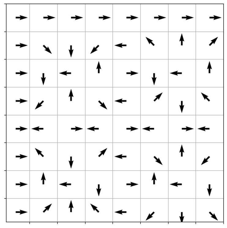
We begin by a special case where n = 8 n = 8 n = 8 M 8 M_8 M 8
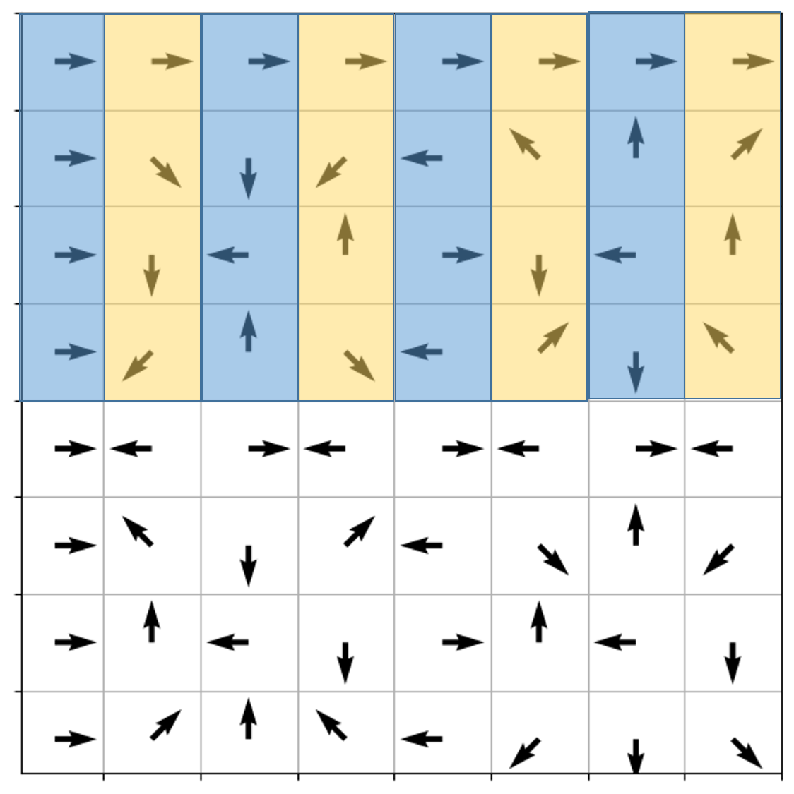
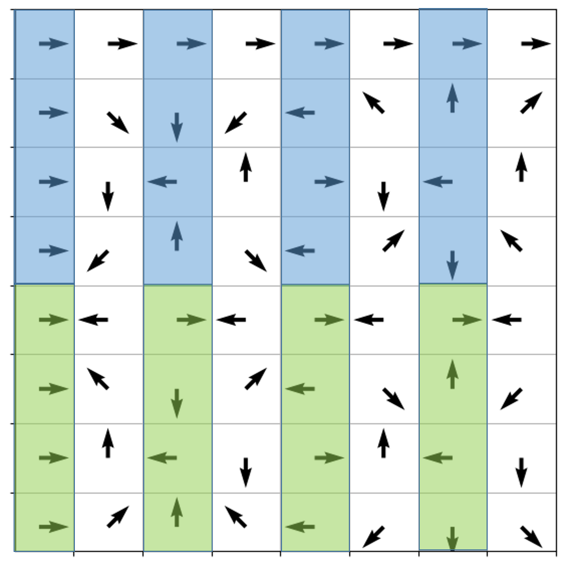
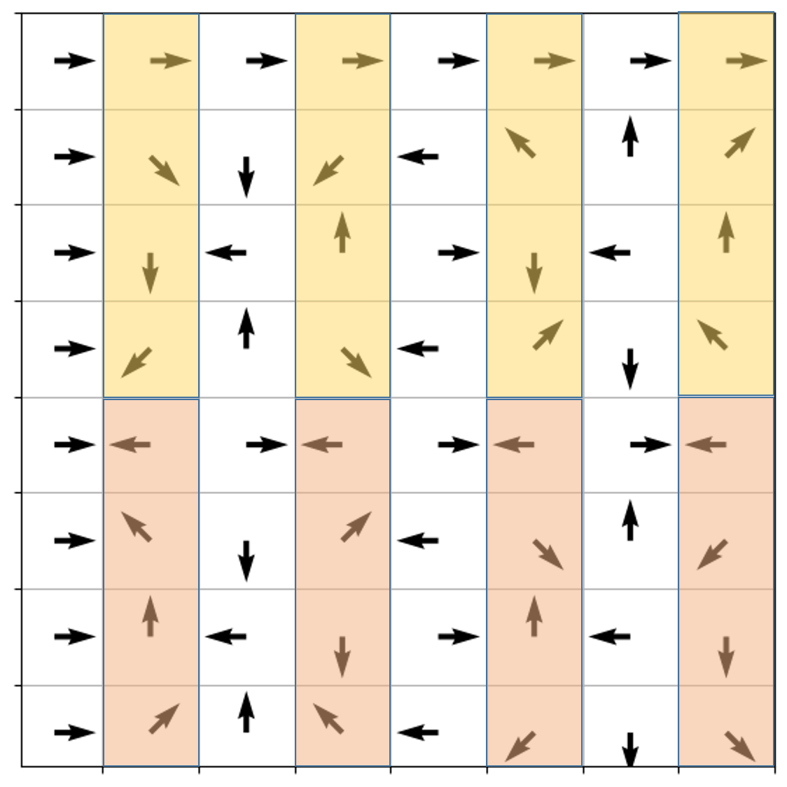
There are some patterns in M 8 M_8 M 8 M 4 M_4 M 4
Remark: I get this visualization idea from [1].
First, look the the first half of the rows of M M M M U M_U M U M 4 M_4 M 4 4 × 4 4 \times 4 4 × 4 M 4 M_4 M 4
Let v e v_e v e v o v_o v o v v v
M U v = M 4 v e + [ e − 2 ⋅ 0 ⋅ π i n e − 2 ⋅ 1 ⋅ π i n e − 2 ⋅ 2 ⋅ π i n e − 2 ⋅ 3 ⋅ π i n ] × M 4 v 0 ,
M_U v = M_4 v_e +
\begin{bmatrix}
e^{ -\frac{2 \cdot 0 \cdot \pi i}{ n} } \\
e^{ -\frac{2 \cdot 1 \cdot \pi i}{ n} } \\
e^{ -\frac{2 \cdot 2 \cdot \pi i}{ n} } \\
e^{ -\frac{2 \cdot 3 \cdot \pi i}{ n} }
\end{bmatrix} \times M_4 v_0,
M U v = M 4 v e + e − n 2 ⋅ 0 ⋅ π i e − n 2 ⋅ 1 ⋅ π i e − n 2 ⋅ 2 ⋅ π i e − n 2 ⋅ 3 ⋅ π i × M 4 v 0 , where × \times ×
M U v = M 4 v e + diag ( e − 2 ⋅ 0 ⋅ π i n , e − 2 ⋅ 1 ⋅ π i n , e − 2 ⋅ 2 ⋅ π i n , e − 2 ⋅ 3 ⋅ π i n ) M 4 v 0 ,
M_U v = M_4 v_e +
\text{diag} \left(
e^{ -\frac{2 \cdot 0 \cdot \pi i}{ n} },
e^{ -\frac{2 \cdot 1 \cdot \pi i}{ n} },
e^{ -\frac{2 \cdot 2 \cdot \pi i}{ n} },
e^{ -\frac{2 \cdot 3 \cdot \pi i}{ n} } \right) M_4 v_0,
M U v = M 4 v e + diag ( e − n 2 ⋅ 0 ⋅ π i , e − n 2 ⋅ 1 ⋅ π i , e − n 2 ⋅ 2 ⋅ π i , e − n 2 ⋅ 3 ⋅ π i ) M 4 v 0 , where diag ( e − 2 ⋅ 0 ⋅ π i n , e − 2 ⋅ 1 ⋅ π i n , e − 2 ⋅ 2 ⋅ π i n , e − 2 ⋅ 3 ⋅ π i n ) \text{diag} \left( e^{ -\frac{2 \cdot 0 \cdot \pi i}{ n} }, e^{ -\frac{2 \cdot 1 \cdot \pi i}{ n} }, e^{ -\frac{2 \cdot 2 \cdot \pi i}{ n} }, e^{ -\frac{2 \cdot 3 \cdot \pi i}{ n} } \right) diag ( e − n 2 ⋅ 0 ⋅ π i , e − n 2 ⋅ 1 ⋅ π i , e − n 2 ⋅ 2 ⋅ π i , e − n 2 ⋅ 3 ⋅ π i ) 4 × 4 4 \times 4 4 × 4
First, look the the second half of the rows of M M M M D M_D M D M 4 M_4 M 4 M U M_U M U
For the odd columns of M D M_D M D M U M_U M U M k , ℓ M_{k, \ell} M k , ℓ M U M_U M U k ∈ [ 0 , n / 2 ) k \in [0, n / 2) k ∈ [ 0 , n /2 ) ℓ \ell ℓ
M k , ℓ = e − ℓ ⋅ ( k − 1 ) ⋅ 2 ⋅ π ⋅ i n .
M_{k, \ell} = e^{ - \ell \cdot (k - 1) \cdot \frac{2 \cdot \pi \cdot i}{n} }.
M k , ℓ = e − ℓ ⋅ ( k − 1 ) ⋅ n 2 ⋅ π ⋅ i . Its corresponding entry in M D M_D M D
M k + n / 2 , ℓ = e − ℓ ⋅ ( k + n / 2 − 1 ) ⋅ 2 ⋅ π ⋅ i n = e − ℓ ⋅ ( k − 1 ) ⋅ 2 ⋅ π ⋅ i n ⋅ e − ℓ ⋅ π ⋅ i = M k , ℓ ⋅ ( − 1 ) .
M_{k + n / 2, \ell} = e^{ - \ell \cdot (k + n / 2- 1) \cdot \frac{2 \cdot \pi \cdot i}{n} } = e^{ - \ell \cdot (k - 1) \cdot \frac{2 \cdot \pi \cdot i}{n} } \cdot e^{ - \ell \cdot \pi \cdot i } = M_{k, \ell} \cdot (-1).
M k + n /2 , ℓ = e − ℓ ⋅ ( k + n /2 − 1 ) ⋅ n 2 ⋅ π ⋅ i = e − ℓ ⋅ ( k − 1 ) ⋅ n 2 ⋅ π ⋅ i ⋅ e − ℓ ⋅ π ⋅ i = M k , ℓ ⋅ ( − 1 ) . The last equality holds since ℓ \ell ℓ
Remark: This also explains why M k + n / 2 , ℓ = M k , ℓ M_{k + n / 2, \ell} = M_{k, \ell} M k + n /2 , ℓ = M k , ℓ ℓ \ell ℓ
In summary, we have
M v = [ M U M D ] v = [ M n / 2 v e + diag ( e − 2 ⋅ 0 ⋅ π i n , e − 2 ⋅ 1 ⋅ π i n , e − 2 ⋅ 2 ⋅ π i n , e − 2 ⋅ 3 ⋅ π i n ) M n / 2 v 0 M n / 2 v e − diag ( e − 2 ⋅ 0 ⋅ π i n , e − 2 ⋅ 1 ⋅ π i n , e − 2 ⋅ 2 ⋅ π i n , e − 2 ⋅ 3 ⋅ π i n ) M n / 2 v 0 ] .
M v
= \begin{bmatrix}
M_U \\
M_D
\end{bmatrix} v
= \begin{bmatrix}
M_{n / 2} v_e +
\text{diag} \left(
e^{ -\frac{2 \cdot 0 \cdot \pi i}{ n} },
e^{ -\frac{2 \cdot 1 \cdot \pi i}{ n} },
e^{ -\frac{2 \cdot 2 \cdot \pi i}{ n} },
e^{ -\frac{2 \cdot 3 \cdot \pi i}{ n} } \right) M_{n / 2} v_0 \\
M_{n / 2} v_e -
\text{diag} \left(
e^{ -\frac{2 \cdot 0 \cdot \pi i}{ n} },
e^{ -\frac{2 \cdot 1 \cdot \pi i}{ n} },
e^{ -\frac{2 \cdot 2 \cdot \pi i}{ n} },
e^{ -\frac{2 \cdot 3 \cdot \pi i}{ n} } \right) M_{n / 2} v_0
\end{bmatrix}.
M v = [ M U M D ] v = M n /2 v e + diag ( e − n 2 ⋅ 0 ⋅ π i , e − n 2 ⋅ 1 ⋅ π i , e − n 2 ⋅ 2 ⋅ π i , e − n 2 ⋅ 3 ⋅ π i ) M n /2 v 0 M n /2 v e − diag ( e − n 2 ⋅ 0 ⋅ π i , e − n 2 ⋅ 1 ⋅ π i , e − n 2 ⋅ 2 ⋅ π i , e − n 2 ⋅ 3 ⋅ π i ) M n /2 v 0 . And the Fast Fourier Transform algorithm is shown as below.
Algorithm FFT (Fast Fourier Transform). Input. v ∈ C n v \in \mathbb{C}^n v ∈ C n
If n = 1 n = 1 n = 1 v v v
Compute r e ← M n / 2 v e r_e \leftarrow M_{n / 2} v_e r e ← M n /2 v e FFT(v e v_e v e .
Compute r o ← M n / 2 v o r_o \leftarrow M_{n / 2} v_o r o ← M n /2 v o FFT(v o v_o v o .
Return
r ← [ r e + diag ( e − 2 ⋅ 0 ⋅ π i n , e − 2 ⋅ 1 ⋅ π i n , e − 2 ⋅ 2 ⋅ π i n , e − 2 ⋅ 3 ⋅ π i n ) r o r e − diag ( e − 2 ⋅ 0 ⋅ π i n , e − 2 ⋅ 1 ⋅ π i n , e − 2 ⋅ 2 ⋅ π i n , e − 2 ⋅ 3 ⋅ π i n ) r o ] .
r \leftarrow
\begin{bmatrix}
r_e +
\text{diag} \left(
e^{ -\frac{2 \cdot 0 \cdot \pi i}{ n} },
e^{ -\frac{2 \cdot 1 \cdot \pi i}{ n} },
e^{ -\frac{2 \cdot 2 \cdot \pi i}{ n} },
e^{ -\frac{2 \cdot 3 \cdot \pi i}{ n} } \right) r_o \\
r_e -
\text{diag} \left(
e^{ -\frac{2 \cdot 0 \cdot \pi i}{ n} },
e^{ -\frac{2 \cdot 1 \cdot \pi i}{ n} },
e^{ -\frac{2 \cdot 2 \cdot \pi i}{ n} },
e^{ -\frac{2 \cdot 3 \cdot \pi i}{ n} } \right) r_o
\end{bmatrix}.
r ← r e + diag ( e − n 2 ⋅ 0 ⋅ π i , e − n 2 ⋅ 1 ⋅ π i , e − n 2 ⋅ 2 ⋅ π i , e − n 2 ⋅ 3 ⋅ π i ) r o r e − diag ( e − n 2 ⋅ 0 ⋅ π i , e − n 2 ⋅ 1 ⋅ π i , e − n 2 ⋅ 2 ⋅ π i , e − n 2 ⋅ 3 ⋅ π i ) r o .
Both step 2 and 3 have time T ( n / 2 ) T(n / 2) T ( n /2 ) O ( n ) O(n) O ( n )
T ( n ) = 2 ⋅ T ( n / 2 ) + O ( n ) .
T(n) = 2 \cdot T(n / 2) + O(n).
T ( n ) = 2 ⋅ T ( n /2 ) + O ( n ) . Reference
[1] T. Roughgarden and G. Valiant, “CS168: The Modern Algorithmic Toolbox Lecture #15 and #16: The Fourier Transform and Convolution,” p. 12.
← Back to all notes Back to top ↑