KLL Sketch

Problem

Let $\mathcal{D}$ be an order domain with size $d$, and $f = (0, \ldots, 0) \in \mathbb{N}^d$ be the frequency vector initialized with all zeros. Suppose that there is a stream $S$ of $n$ elements updating $f$ as follows:

For each $x \in S$ do
$\qquad$ $f[x] \leftarrow f[x] + 1$.

When all updates in $S$ have arrived, we have that $|S| = \Vert f \Vert_1 = n$.

We study the ranks of elements in $\mathcal{D}$.

Definition. For $x \in \mathcal{D}$, define the rank $r(x)$ of $x$ to as

$$r(x) \doteq \sum_{y < x} f[y].$$

Approximate Rank Query. Given a parameter $\epsilon \in (0, 1)$, design a data structure which, for each $x \in \mathcal{D}$, outputs an estimate $\hat r(x)$ of $r(x)$, such that

$$r(x) - \epsilon \Vert f \Vert_1 \le \hat r(x) \le r(x) + \epsilon \Vert f \Vert_1.$$

MRL Sketch

Theorem (MRL Sketch). If the size of the stream $|S| = n$ is given in advance, the MRL Sketch solves the approximate rank query with space usage

$$O \left( \epsilon^{-1} \log^2 (\epsilon n) \right).$$

Structure

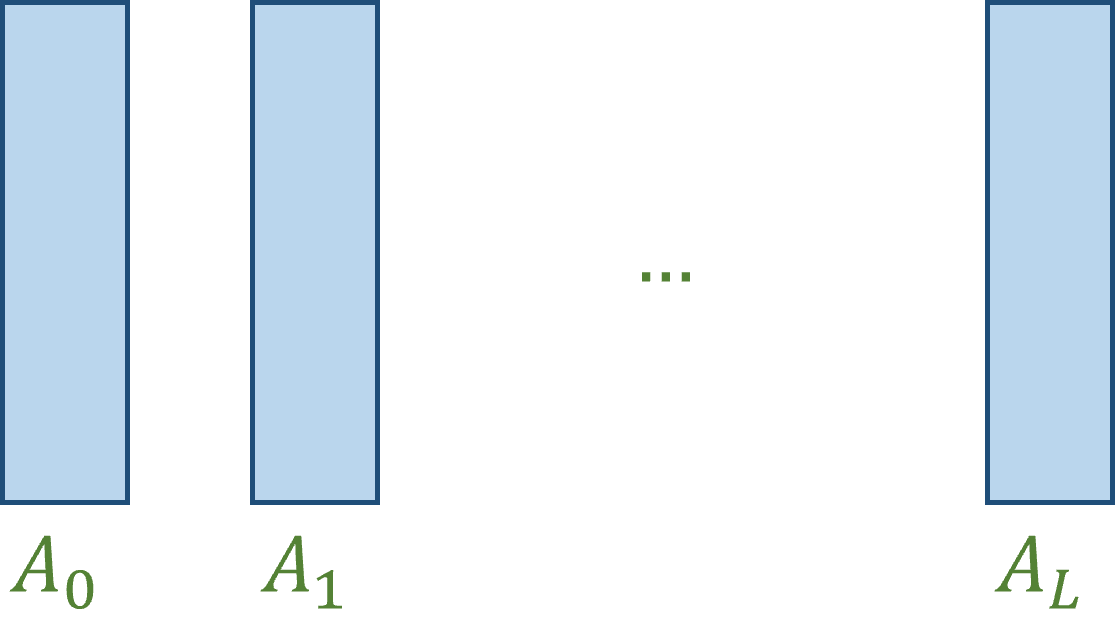
The structure of the algorithm comprises a sequence of $L + 1$ arrays $A_0, \ldots A_L$, each of size

where $\lceil \cdot \rceil_{even}$ is the operation of rounding a real number up to nearest even integer.

It sets $L$, the largest index of the arrays, to $\lceil \log (n / k) \rceil$. Therefore,

Insertion

The MRL sketch processes an insertion as follows.

Insert: $x \in \mathcal{D}$.

1. Insert $x$ into $A_0$;
2. COMPRESS.

The algorithm COMPRESS inspects the arrays $A_0, \ldots, A_{L - 1}$ in increasing order. If an array $A_i$, reaches its capacity, the algorithm performs a compaction on $A_i$. In particular, it moves the odd-indexed elements of $A_i$ to $A_{i + 1}$, and then reset $A_i$ to empty (by deleting all its elements). This may cause $A_{i + 1}$ to research its capacity, and trigger a sequence of compactions.

COMPRESS.

1. $i \leftarrow 0$;
2. while $i < L$ and $|A_i| = k:$ // no empty buckets
3. $\qquad$ Sort $A_i$ in increasing order.
4. $\qquad$ Move $A_i[1], A_i[3], \ldots, A_i[k - 1]$ into $A_{i + 1}$
5. $\qquad$ Delete all elements in $A_i$
6. $\qquad$ $i \leftarrow i + 1$.

Suppose that each elements in array $A_i$ ($0 \le i \le L$) is associated with weight $w_i = 2^i$. It is easy to prove, by induction on the size of $n$, and on the number of inductions performed, the following invariant

Invariant. For $0 \le i \le L$, define $w_i = 2^i$. Then

$$\sum_{ i = 0}^L w_i \cdot |A_i| = n.$$

Therefore, $2^L |A_L| = 2^{ \lceil \log (n / k) \rceil } \cdot |A_L| \le n$. Therefore, $|A_L| \le k$ and $A_L$ will never exceed its capacity.

Interpretation of Weights

The weights have another interpretation. Suppose that we associate each element inserted into $A_0$ with a set, which contains only the element itself. We will maintain these sets, such that

For each $0 \le i \le L$, and each $v \in A_i$, the set associated with $v$ has size $w_i$, and $v$ is the only element in the set that is kept in the arrays. Further, the sets associated with different elements in the arrays are disjoint.

Clearly this holds when an element is inserted into $A_0$. Now, suppose we are going to perform a compaction at an array $A_i$, for some $0 \le i < L$. We delete half of the elements in $A_i$, and keep the rest of the elements. We can pair up the elements deleted and the ones kept one by one, and merge their associated sets. For each merged set, it contains $w_{i + 1}$ elements, and only one element in the merge set is kept in the arrays. Hence, we can associate it with the only element kept.

The above discussion gives a new interpretation of the weights.

If an element is associated with weight $w_i$, it represents $w_i$ unique elements in the original stream.

Query

Definition. For each $i \in \{0, \ldots, L \}$, and $x \in \mathcal{D}$, let $r(x, A_i)$ be the rank of $x$ in $A_i$, defined as

$$r(x, A_i) \doteq | \{ y \in A_i : y < x \} |,$$

which is the number of elements in $A_i$ that is strictly less than $x$.

Given $x \in D$, the MRL sketch returns an weighted sum of the ranks $r(x, A_i)$, as an estimate of $r(x)$:

Rank: $x \in \mathcal{D}$

1. $\hat r(x) \leftarrow 0$;
2. For $i \leftarrow 0$ to $L$ do
3. $\qquad$ $\hat r(x) \leftarrow \hat r(x) + w_i \cdot r(x, A_i)$.

Error Analysis

Now we analyze the approximation error of $\hat r(x)$.

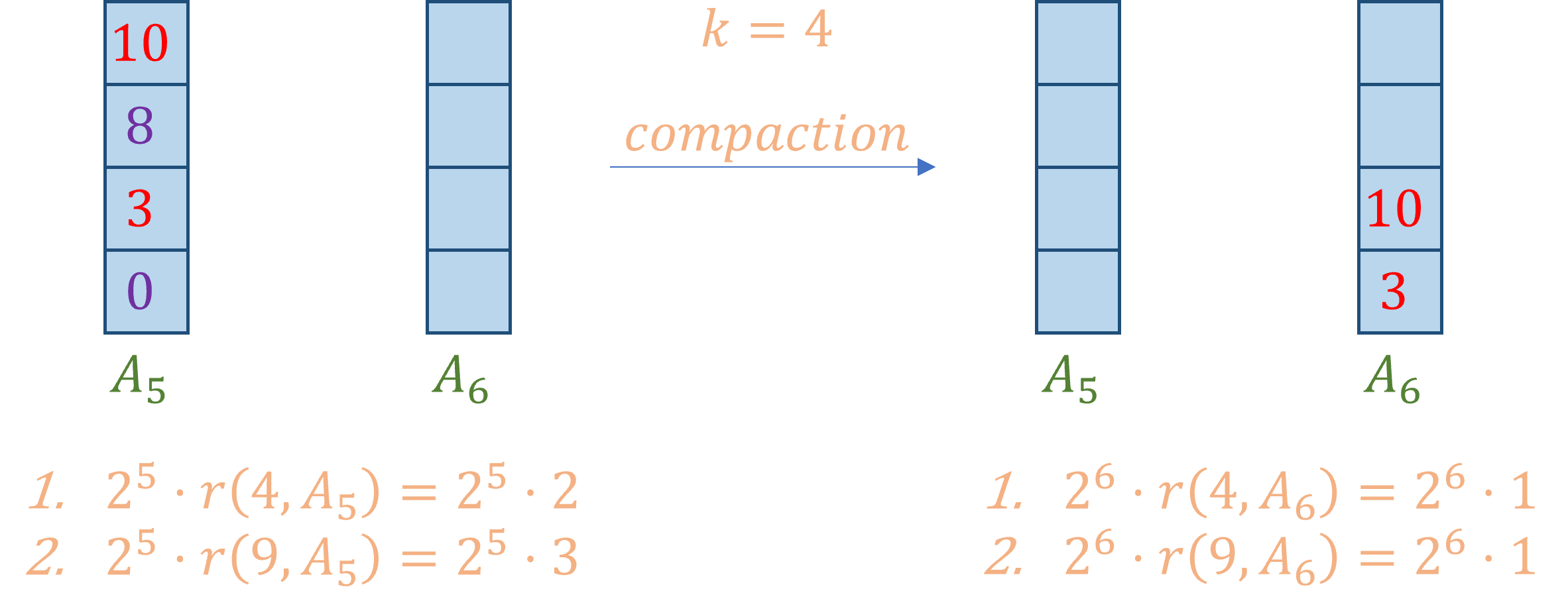
We illustrate the key idea of the analysis via an example. In the figure below, $k = 4$. Before the compaction, $A_5$ contributes $2^5 \cdot r(4, A_5) = 2^5 \cdot 2$ to the estimation of $\hat r(4)$, and $2^5 \cdot r(9, A_5) = 2^5 \cdot 3$ to the estimation of $\hat r(9)$.

The compaction moves elements in the odd positions of $A_5$, namely $3$ and $10$, to $A_6$. Then it deletes all elements in $A_5$.

After the compaction, $A_6$ contributes $2^6 \cdot r(4, A_6) = 2^6 \cdot 1$ to the estimation of $\hat r(4)$, and $2^6 \cdot r(9, A_6) = 2^6 \cdot 1$ to the estimation of $\hat r(9)$.

There is no error incurred to the estimation of $\hat r(4)$ at this compaction step, while the estimation error incurred to $\hat r(9)$ is $-2^5$ at this compaction step.

The above discussion leads to the following observations.

Observation. Let $x \in \mathcal{D}$ and $0 \le i < L$. Denote $A_i, A_{i + 1}$ the arrays before the compaction and $A_i', A_{i + 1}'$ the ones after.

1. If $r(x, A_i)$ is even, then

   $$w_{i + 1} \cdot r(x, A_{i + 1}' ) = w_{i + 1} \cdot r(x, A_{i + 1} ) + w_{i} \cdot r(x, A_i),$$

   which implies that the compaction at $A_i$ incurs no error to the estimation of $r(x)$.

2. If $r(x, A_i)$ is odd, then

   $$w_{i + 1} \cdot r(x, A_{i + 1}' ) + w_i = w_{i + 1} \cdot r(x, A_{i + 1} ) + w_{i} \cdot r(x, A_i).$$

   which implies that the compaction at $A_i$ incurs an error of $-2^i$ to the estimation of $r(x)$.

Let $m_i$ be the number of compactions performed at $A_i$. For each $j < i$, each compaction at $A_j$ discards $k / 2$ elements and transfers only $k / 2$ elements to $A_{j + 1}$. Therefore, the number of elements that have ever been inserted into $A_i$ is bounded by $n / 2^i$, and $m_i$ is bounded by

Given $x \in \mathcal{D}$, let $\eta_{i, t}$ be the parity of $r(x, A_i)$ just before the $t^{(th)}$ compaction is performed on $A_i$. The estimation error $\mathbb{Err}(x)$ is given by

The last inequality follows from that $L / k \le \epsilon$.

Basic KLL Sketch

In this section, we reduce the space usage from $O \left( \epsilon^{-1} \cdot \log^2 (\epsilon n) \right)$ to

The algorithm is a randomized one and has failure probability $\delta$.

The algorithm is similar to the MRL sketch, but sets $k = 2 / \epsilon \cdot \sqrt{ \ln 2 / \delta }$ and $L = \lceil \log (n / k) \rceil$ to achieve the space usage stated above. Besides, the compaction step is different.

Random Parity

Instead of always moving the odd-indexed elements to the next array, it chooses uniformly at random either the odd-indexed elements, or even-indexed elements. In particular, it replaces the line 4 of the COMPRESS algorithm with the following lines:

1. Flip an unbiased coin;
2. If the coin turns out head:
3. $\qquad$ Move $A_i[1], A_i[3], \ldots, A_i[k - 1]$ into $A_{i + 1}$;
4. Else:
5. $\qquad$ Move $A_i[0], A_i[2], \ldots, A_i[k - 2]$ into $A_{i + 1}$;

Unbiased Estimation

For each $x \in \mathcal{D}$ and $0 \le i < L$, if $r(x, A_i)$ is even, then there is no error introduced after the compaction on $A_i$. If $r(x, A_i)$ is odd, then the error introduced is either $2^i$ or $-2^i$, both with probability $1 / 2$. Hence, the expected error is always $0$.

The estimation error $\mathbb{Err}(x)$ is given by

where $\sigma_{i, t} \in \{-1, 1\}$ are Rademacher random variables.

Clearly, we have that

Confidence Interval of the Estimation Error

However, the random variables $\eta_{i, t} \cdot \sigma_{i, t} \cdot 2^i$ are not independent, as the values of $\eta_{i, t}$ depends on previous compressions.

Instead of using the Hoeffding's inequality for independent random variables, we resort to a martingale concentration inequality.

Martingale Difference Sequence

Let $m = \sum_{ i = 0}^{L - 1} m_i$ be the total number of compaction at the arrays. For fixed $n$ and $k$, $m$ is a deterministic number (even without knowing the elements in $S$). Further, for each $t \in [m]$, the array at which the $t$-th compaction is performed is also deterministic. Denote $a_t \in [0, \ldots, L - 1]$ the index of the corresponding array, and let $c_t \doteq 2^{ a_t }$, which is a deterministic number since $a_t$ is deterministic. It holds that

The last inequality follows since $L = \lceil \log (n / k) \rceil$.

For each $t \in [m]$, define the random variable $X_t \in \{-c_t, 0, c_t\}$, such that

1. If $rank(x, A_{a_t})$ is even, then $\Pr[ X_t = 0] = 1$.
2. If $rank(x, A_{a_t})$ is odd, then $\Pr[ X_t = -c_t ] = \Pr[ X_t = c_t ] = 1 / 2$

The $X_t$ are not independent random variables, since for $t > 1$, when the $t$-th compaction happens at the $a_t$-th array $A_{a_t}$, the rank of $x$ at this array depends on the previous compressions. However, the conditional expectation of $X_t$ is always $0$:

Hence, $X_1, \ldots, X_m$ is a martingale difference sequence.

Theorem.([1]) Let $c_1, \ldots, c_m$ be constants, and let $X_1, \ldots, X_m$ be a martingale difference sequence with $|X_t| \le c_t$ for each $t$. Then for any $\lambda \ge 0$,

$${ \small \Pr \left[ \left| \sum_{t \in [m] } X_t \right| \ge \lambda \right] \le 2 \cdot \exp \left( - \frac{ \lambda^2 }{ 2 \cdot \sum_{ t \in [m] } c_t^2 }\right). }$$

Choosing $k$

It follows that with probability at least $1 - \delta$, it holds that

Setting $k = \Big\lceil 2 / \epsilon \cdot \sqrt{ \ln 2 / \delta } \Big\rceil_{even}$, this error is bounded by $\epsilon \cdot n$.

The total space usage is therefore

Remark. It is kind of amazing that the size of $k$ does not depends on $n$. On the other hand, even though the size of $L$ depends on $n$, we can still apply the algorithm when we don't know the value of $n$ in advance. We can create new arrays on the fly. In particular, if the array with the largest index exceeds its capacity, we perform compaction at it and create a new array. Note the we don't perform compaction at that array, when it reaches its capacity. The entire analysis still holds.

Improved KLL Sketch

In this section, we improve the space usage to

Compared to the basic KLL, the improved algorithm allows the capacities of the arrays to vary. Denote the largest index of the arrays as $L$. It and maintains the following invariant:

• For each $0 \le i \le L$, the array $A_{L - i}$ has capacity $\lceil \alpha^i \cdot k \rceil_{even}$, where $\alpha \in (0.5, 1)$ is a parameter chosen by the algorithm.

The algorithm sets $k = \Big\lceil 2 / \epsilon \cdot \sqrt{ 1 / (2 \alpha - 1 ) \cdot \ln 2 / \delta } \Big\rceil_{even}$. When $n$ elements arrive, at least one compaction is performed at $A_{L - 1}$, as otherwise $A_L$ would be not created. When the first compaction is performed at $A_{L - 1}$, it has capacity $k$. As each element in $A_{L - 1}$ represents $2^{L - 1}$ unique elements in the original stream,

It follows that the total space usage is bounded by

If we set, e.g., $\alpha = 2 / 3$, then this is

Algorithm

Initially, $L = 0$ and the algorithm creates a single array $A_0$ with capacity $k$. When $A_L$ reaches or exceeds its capacity, the algorithm increases $L$ and creates a new array. The new algorithm COMPRESS is as follows.

COMPRESS.

1. $i \leftarrow 0$
2. while $|A_i| \ge \lceil \alpha^{L - i} \cdot k \rceil_{even}$ // no empty buckets
3. $\qquad$ If $i = L$ then
4. $\qquad\qquad$ $L \leftarrow L + 1$
5. $\qquad\qquad$ Create a new array $A_L$
6. $\qquad$ Sort $A_i$ in increasing order
7. $\qquad$ Flip an unbiased coin
8. $\qquad$ If $A_i$ contains odd number of elements then
9. $\qquad$ $\qquad$ $E \leftarrow$ the element at the back of $A$
10. $\qquad$ $\qquad$ delete $E$ from $A$
11. $\qquad$ Else
12. $\qquad$ $\qquad$ $E \leftarrow$ null
13. $\qquad$ If the coin turns out head then
14. $\qquad$ $\qquad$ Move odd index elements of $A_i$ to $A_{ i + 1 }$
15. $\qquad$ Else:
16. $\qquad$ $\qquad$ Move even index elements of $A_i$ to $A_{i + 1}$
17. $\qquad$ Delete all elements in $A_i$
18. $\qquad$ If $E \neq$ null then
19. $\qquad$ $\qquad$ Put $E$ back into $A_i$
20. $\qquad$ $i \leftarrow i + 1$

Analysis

Maintaining the Invariant

Lemma. The invariant is maintained.

Proof. We prove this by induction. Initially, $L = 0$ and $A_0$ has capacity $k$. If $A_0$ has not reaches its capacity, the invariant holds trivially.

Now, suppose that the invariant holds before the algorithm COMPRESS.

If $L$ is not increased and no new array is created by the algorithm, i.e., the while loop of the algorithm stops for $i \le L$, then the invariant still holds.

If $L$ is increased and new arrays are created, then when the algorithm COMPRESS stops, compactions have been performed for all arrays except the one with highest index. Hence, $ 0 \le |A_j| \le 1 < \lceil \alpha^i \cdot k \rceil_{even}. $ Finally, when while loop stops, it holds that $i = L$. The stopping condition implies that $|A_L| < \lceil \alpha^0 \cdot k \rceil_{even} = k$.

$\square$

Question to ponder: Prove that at most one new array can be created by COMPRESS each time it is invoked.

Bounding the Number of Compaction

Lemma. When the algorithms stops, for each $i \in [L]$, the number of compaction performed at the array $A_{L - i}$ is bounded by $(4 / \alpha)^i$.

Proof. For each $i \in [L]$, when a compaction is performed at $A_{L - i}$, at least $\lceil \alpha^i \cdot k \rceil_{even}$ elements are removed from it. As each element in $A_{L - i}$ represents $2^{L - i}$ elements in the original stream, it holds that

$\square$

Finally, we discuss the estimation error of an element. For fixed $n$, the number of compactions performed, as well as the order of the compactions performed are deterministic. Using the notations in the previous section, we have

Using that $2^{L - 1} \le \frac{n}{k}$, and that

we see

It follows that with probability at least $1 - \delta$, it holds that

Setting $k = \Big\lceil 2 / \epsilon \cdot \sqrt{ \frac{1}{2 \alpha - 1} \cdot \ln 2 / \delta } \Big\rceil_{even}$, this error is bounded by $\epsilon \cdot n$.

Reference

[1] C. McDiarmid, “Concentration,” in Probabilistic Methods for Algorithmic Discrete Mathematics, M. Habib, C. McDiarmid, J. Ramirez-Alfonsin, and B. Reed, Eds. Berlin, Heidelberg: Springer Berlin Heidelberg, 1998, pp. 195–248.

[2] Z. Karnin, K. Lang, and E. Liberty, “Optimal Quantile Approximation in Streams,” arXiv:1603.05346 [cs], Apr. 2016